Difference between revisions of "DNA Melting: Simulating DNA Melting - Basics"
Steven Nagle (Talk | contribs) |
Eliot Frank (Talk | contribs) |
||
| Line 49: | Line 49: | ||
</math> | </math> | ||
| − | where ''C_T'' is the total concentration of DNA strands. | + | where ''<math>C_T</math>'' is the total concentration of DNA strands. |
Since this is a complicated equation that we will evaluate many times, it makes sense to write a Matlab function. | Since this is a complicated equation that we will evaluate many times, it makes sense to write a Matlab function. | ||
| Line 125: | Line 125: | ||
Experiment with different values of ''ΔS°'' and ''ΔH°'' to see how the curve changes. | Experiment with different values of ''ΔS°'' and ''ΔH°'' to see how the curve changes. | ||
| − | + | Several web tools are available to predict the melting temperature as well as ''ΔS°'' and ''ΔH°''. See, for example, [http://mfold.rna.albany.edu/?q=DINAMelt/Hybrid2 DINA Melt] or [http://www.basic.northwestern.edu/biotools/oligocalc.html Oligocalc]. You can use one of these or another tool to estimate values for different DNA sequences. | |
| + | The DNA sequences used in the lab are listed at [[DNA Melting: DNA Sequences]]. For DNA Melting Part I, you will be using a 20 base pair sequence ("20bp" and its complement "20bp-comp") at 30μM concentration in a 100mM saline solution. Try plugging in the 20bp sequence (or other sequence listed) into DINA Melt and/or Oligocalc to get estimates of the thermodynamic parameters. | ||
One method of estimating ''T<sub>m</sub>'' is to find the temperature where the dsDNA fraction equals 1/2. Another method is to differentiate the melting curve. ''T<sub>m</sub>'' occurs at the peak of the derivative — where the dsDNA fraction is changing the fastest. (Why might you prefer one method over the other when estimating ''T<sub>m</sub>'' from experimental data?) | One method of estimating ''T<sub>m</sub>'' is to find the temperature where the dsDNA fraction equals 1/2. Another method is to differentiate the melting curve. ''T<sub>m</sub>'' occurs at the peak of the derivative — where the dsDNA fraction is changing the fastest. (Why might you prefer one method over the other when estimating ''T<sub>m</sub>'' from experimental data?) | ||
| Line 188: | Line 189: | ||
:''T<sub>i</sub>'' is the initial temperature, likely room temperature, | :''T<sub>i</sub>'' is the initial temperature, likely room temperature, | ||
:''T<sub>max</sub>'' is the max temperature reached during the heating phase, | :''T<sub>max</sub>'' is the max temperature reached during the heating phase, | ||
| − | :''T<sub>f</sub>'' is the final temperature, likely | + | :''T<sub>f</sub>'' is the final temperature, likely room temperature, |
| − | :''τ'' | + | :''τ<sub>HT</sub>'' and ''τ<sub>CL</sub>'' are the time constants for heating (HT) and cooling (CL). |
In Matlab: | In Matlab: | ||
| Line 195: | Line 196: | ||
<pre> | <pre> | ||
sim1.heatingConstant = 180; % heating rate constant, 1/s | sim1.heatingConstant = 180; % heating rate constant, 1/s | ||
| − | sim1.coolingConstant = | + | sim1.coolingConstant = 300; % cooling rate constant, 1/s |
sim1.maxTemperature = 95 + 273; % target maximum sample temp, K | sim1.maxTemperature = 95 + 273; % target maximum sample temp, K | ||
sim1.initialTemperature = 20 + 273; % starting room temp, K | sim1.initialTemperature = 20 + 273; % starting room temp, K | ||
| − | sim1.finalTemperature = | + | sim1.finalTemperature = 20 + 273; % final cool-down temp, K |
% use exp function to model exponential heating and cooling | % use exp function to model exponential heating and cooling | ||
| Line 269: | Line 270: | ||
[[Image:SimDNAFractionCurve.png|350px|Simulated DNA Melting Curve]] | [[Image:SimDNAFractionCurve.png|350px|Simulated DNA Melting Curve]] | ||
| − | |||
| − | |||
| − | |||
| − | |||
| − | |||
| − | |||
| − | |||
| − | |||
| − | |||
| − | |||
| − | |||
| − | |||
| − | |||
| − | |||
| − | |||
| − | |||
| − | |||
| − | |||
| − | |||
| − | |||
| − | |||
| − | |||
| − | |||
| − | |||
| − | |||
| − | |||
| − | |||
| − | |||
| − | |||
| − | |||
| − | |||
| − | |||
| − | |||
| − | |||
| − | |||
| − | |||
| − | |||
| − | |||
| − | |||
| − | |||
| − | |||
| − | |||
| − | |||
| − | |||
| − | |||
| − | |||
| − | |||
| − | |||
==Issues experienced in practice== | ==Issues experienced in practice== | ||
| Line 360: | Line 313: | ||
noise = 0.01 * randn(1,length(sim1.V_f))'; % Random noise, standard deviation=10mV | noise = 0.01 * randn(1,length(sim1.V_f))'; % Random noise, standard deviation=10mV | ||
sim1.V_f = sim1.V_f + noise; % Add random noise | sim1.V_f = sim1.V_f + noise; % Add random noise | ||
| − | |||
| − | |||
| − | |||
| − | |||
figure(9) | figure(9) | ||
| Line 378: | Line 327: | ||
Here too you are encouraged to add noise at additional frequencies that you think might be present in the lab. What could you do to minimize the effects of these noise sources? Think of solutions both at the hardware level and at the software level and model both of them. | Here too you are encouraged to add noise at additional frequencies that you think might be present in the lab. What could you do to minimize the effects of these noise sources? Think of solutions both at the hardware level and at the software level and model both of them. | ||
| − | |||
| − | |||
| − | |||
| − | |||
| − | |||
| − | |||
| − | |||
| − | |||
| − | |||
| − | |||
| − | |||
| − | |||
| − | |||
| − | |||
| − | |||
| − | |||
| − | |||
| − | |||
| − | |||
| − | |||
| − | |||
| − | |||
| − | |||
| − | |||
| − | |||
| − | |||
| − | |||
| − | |||
| − | |||
| − | |||
| − | |||
| − | |||
| − | |||
| − | |||
| − | |||
| − | |||
==Lab manual sections== | ==Lab manual sections== | ||
Revision as of 17:01, 8 August 2013
Introduction
Chance favors the prepared mind.
—Louis Pasteur (abridged)
This tutorial will show you how to simulate the DNA melting experiment with Matlab. The DNA melting apparatus you will build produces two output voltages related to the sample temperature and fluorescence intensity. During an experimental run, these two voltages will be recorded periodically. At the end of this tutorial, you will be able to produce mock datasets that are similar to what you will record in the lab. You can use simulated datasets to help develop and debug your data analysis scripts.
It is essential to have working data analysis scripts before you begin running experiments in the lab.
The procedure for creating the simulation is:
- Write a function to compute the equilibrium dsDNA concentration vs. temperature
- Model sample temperature versus time during an experimental run
- Compute the RTD voltage from temperature vs. time data
- Compute relative fluorescence intensity vs. time data from temperature vs. time data
Run Matlab and follow along as you read. Code from this page can be copied and pasted into the Matlab command window.
If you prefer to work in Python, please see this page.
Before you begin
- Review the DNA Melting Thermodynamics Notes.
- If you need a review of Matlab fundamentals, see Matlab Fundamentals tutorial.
Matlab skills
- Array arithmetic (element-by-element) operators (+, -, .*, ./)
- Functions declared in an m-file
- Conditionals
- Functions that take a variable number of arguments
- Numerical differentiation
- Plotting data
Modeling dsDNA equilibrium fraction
We derived an expression for dsDNA fraction at a given temperature in class:
- $ K_{eq} = e^\left [\frac{\Delta S^{\circ}}{R} - \frac{\Delta H^{\circ}}{R T} \right ] $
- $ f = \frac{1 + C_T K_{eq} - \sqrt{1 + 2 C_T K_{eq}}}{C_T K_{eq}} $
where $ C_T $ is the total concentration of DNA strands.
Since this is a complicated equation that we will evaluate many times, it makes sense to write a Matlab function.
dsDNA fraction function
The fraction of dsDNA is a function of 4 variables: ΔS°, ΔH°, temperature, and concentration. The DnaFraction function below also takes an optional fifth argument for the gas constant to enable using different unit systems. Using the element-by-element divide operator in the body of the function makes it possible for DnaFraction to accept either a single temperature argument or a vector of temperature values. (As a general rule, use the ./ operator instead of / unless you intend to do a matrix divide.)
The Matlab function nargin returns the number of arguments that the function was called with. Many Matlab programs use this function to handle variable numbers of arguments. If nargin returns 4 or less, R is set to the default value of 1.987. Otherwise, the value of R is set to the value supplied by the caller.
Matlab notes: Matlab functions must be saved in the current directory or another directory in the Matlab path. The name of the file must be the function name appended with ".m". Function help should be placed in comments at the top of the file. Type help DnaFraction to see how this works.
% Returns the fraction of dsDNA in a solution containing equal concentrations
% of two complementary DNA oligos as a functino of total DNA concentration,
% temperature, entropy change, and enthalpy change.
% Gas constant is an optional parameter.
%
% USAGE: f = DnaFraction(Ct, T, DeltaS, DeltaH, <GasConstant>)
% RETURN VALUE: fraction of dsDNA
%
% Default units are molar, Kelvin, cal/mole, and cal/(mole-Kelvin). For
% other unit systems, supply the appropriate value of R in the optional
% fifth parameter. The default value is 1.987 cal/(degree K * mole).

function f = DnaFraction(Ct, T, DeltaS, DeltaH, GasConstant)
% Gas constant
if(nargin < 5)              % determine if caller supplied R value or not
    R = 1.987;              % set to default: cal/(degree K * mole)
else
    R = GasConstant;        % otherwise use caller's value
end

% Compute Ct * Keq
CtKeq = Ct * exp(DeltaS / R - DeltaH ./ (R * T));

%now compute f
f = (1 + CtKeq - sqrt(1 + 2 * CtKeq)) ./ CtKeq;

% Written 4/9/2008 by SCW
Plot an ideal melting curve
Does the DnaFraction function work as expected? A good way to test the function is to plot a melting curve generated by DnaFraction.
Matlab notes: Over the course of an interactive Matlab session, you may run several simulations with different parameters. Using a structure to keep the results of each simulation together is a good way to prevent the workspace from becoming disorganized. The struct function creates an empty structure. In the code below, a structure called ideal is created to hold the ideal melting curve data. (Since variables are dynamically allocated and typed in Matlab, the struct command is optional; however, explicitly creating the structure can make your code easier to read and better performing.)
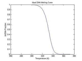
Since DnaFraction accepts a vector temperature argument, an entire melting curve can be computed with a single call.
close all;
clc;

ideal = struct();                          % create an empty structure to hold the results
ideal.temperature = (0:99) + 273.15;       % temperature axis in Kelvin: 100 points(0-99C)
ideal.deltaS = -184;                       % cal/mol
ideal.deltaH = -71E3;                      % cal/(mol K)
ideal.DnaConcentration = 30E-6;            % M

% call DnaFraction function
% arguments: concentration, temperature vector, delta S, delta H
% (optional R argument not supplied)

ideal.dsDnaFraction = DnaFraction(ideal.DnaConcentration, ...
    ideal.temperature, ideal.deltaS, ideal.deltaH);

figure(1)
plot(ideal.temperature, ideal.dsDnaFraction);
title('Ideal DNA Melting Curve');
xlabel('Temperature (K)');
ylabel('dsDNA Fraction');
Experiment with different values of ΔS° and ΔH° to see how the curve changes.
Several web tools are available to predict the melting temperature as well as ΔS° and ΔH°. See, for example, DINA Melt or Oligocalc. You can use one of these or another tool to estimate values for different DNA sequences. The DNA sequences used in the lab are listed at DNA Melting: DNA Sequences. For DNA Melting Part I, you will be using a 20 base pair sequence ("20bp" and its complement "20bp-comp") at 30μM concentration in a 100mM saline solution. Try plugging in the 20bp sequence (or other sequence listed) into DINA Melt and/or Oligocalc to get estimates of the thermodynamic parameters.
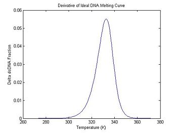
One method of estimating Tm is to find the temperature where the dsDNA fraction equals 1/2. Another method is to differentiate the melting curve. Tm occurs at the peak of the derivative — where the dsDNA fraction is changing the fastest. (Why might you prefer one method over the other when estimating Tm from experimental data?)
Numerical differentiation
The fluorescence function fN is a sampled version of the continuous function f(T) such that fN = f(NΔT), where ΔT is the sampling interval (1° C, in this instance). One method for computing a numerical approximation to df/dT is the finite difference:
- $ {f'}_N = \frac{f_{N+1}-f_{N}}{\Delta T} $.
df/dT is guaranteed to take on the value given by f'N at some point between NΔT and (N+1)ΔT; however, this happy coincidence can occur at any place in the interval. A simple but effective technique is to guess that equality occurs in the middle of the interval. This guess is close enough in most cases.
The code below computes the finite difference and stores it in the dDsDnaFraction field of ideal. It also generates an associated temperature vector (ideal.dTemperature) with values centered between the original temperature samples. Note that both vectors are one element shorter than the original data.
ideal.dTemperature = ideal.temperature(1:99) + 0.5; % create new temperature vector
ideal.dDsDnaFraction = diff(ideal.dsDnaFraction);   % take adjacent element differences

figure(2)
plot(ideal.dTemperature, -1 * ideal.dDsDnaFraction);
title('Derivative of Ideal DNA Melting Curve');
xlabel('Temperature (K)');
ylabel('Delta dsDNA Fraction');
In the previous section, the plot shows that the dsDNA fraction equals 0.5 at about 332.5 degrees. The peak of the derivative also occurs at the same temperature. (The curve is plotted inverted.)
Set up simulation conditions and data structure
It will be convenient to set up a data structure with the simulation parameters and a time axis.
sim1 = struct();                                          % create empty struct for sim results
sim1.DnaConcentration = 30E-6;                            % 30 micromolar concentration
sim1.deltaS = ideal.deltaS;                               % cal / (mole-K)
sim1.deltaH = ideal.deltaH;                               % cal / mole
sim1.finalTemperature = 293;                              % approx. room temperature
sim1.sampleRate = 1;                                      % 1 Hz sample rate
sim1.durationHT = 900;                                    % heating time, s
sim1.durationCL = 600;                                    % cooling time, s
sim1.timeHT = (0:(1/sim1.sampleRate):sim1.durationHT)';   % heating time vector, s
sim1.timeCL = (2:(1/sim1.sampleRate):sim1.durationCL)';   % cooling time vector, s
sim1.time = [sim1.timeHT; sim1.timeHT(end)+sim1.timeCL];  % complete time vector, s
Simulate sample temperature during an experimental run
The goal of the simulation is to produce two simulated voltage signals that resemble what you will measure in the lab. Since both of the voltages are functions of temperature, it makes sense to begin by modeling how the sample temperature behaves during an experimental run.
Sample heating and cooling
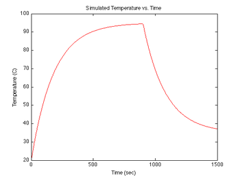
During each experimental run, the range of temperatures will be provided by forced heating by a TEC, followed by natural cooling of the sample after the heat source is switched off. At the beginning of an experimental run the sample will be at room temperature, then the TEC is switched on and the DNA + fluorescent dye sample is heated to 95°C in about 5 minutes. Upon reaching 95°C, the TEC power is switched off. Then over a period of about 15 minutes, the sample cools to room temperature (less than 30°C). The rate of cooling is proportional to the difference between the sample's temperature and the room temperature, so the sample cools more quickly at the start of the experiment than near the end. (It can be frustrating to wait for the final few degrees.)
Both heating and cooling can be approximated by an exponential function. Heating is modeled with a time constant of about 1 minute, while cooling is modeled with a time constant of about 3 minutes. The equation for temperature (in K) versus time is:
- $ T_{heating}(t) = (T_{max} - T_i) (1 - e ^ {-\frac{t_{HT}}{\tau_{HT}}}) + T_i $
- $ T_{cooling}(t) = (T_{max} - T_f) e ^ {-\frac{t_{CL}}{\tau_{CL}}} + T_f $
where,
- T(t) is the temperature as a function of time,
- Ti is the initial temperature, likely room temperature,
- Tmax is the max temperature reached during the heating phase,
- Tf is the final temperature, likely room temperature,
- τHT and τCL are the time constants for heating (HT) and cooling (CL).
In Matlab:
sim1.heatingConstant = 180;                               % heating rate constant, 1/s
sim1.coolingConstant = 300;                               % cooling rate constant, 1/s
sim1.maxTemperature = 95 + 273;                           % target maximum sample temp, K
sim1.initialTemperature = 20 + 273;                       % starting room temp, K
sim1.finalTemperature = 20 + 273;                         % final cool-down temp, K

% use exp function to model exponential heating and cooling
sim1.temperature = ...
    [ (sim1.maxTemperature - sim1.initialTemperature)   ... % (T_max - T_i) *
    .* (1 - exp(-sim1.timeHT ./ sim1.heatingConstant))  ... % (1 + e^(-t/tauHT)) +
    + sim1.initialTemperature; ...                          % T_i
    (sim1.maxTemperature - sim1.finalTemperature)   ...     % (T_max - T_f) *
    .* exp(-sim1.timeCL ./ sim1.coolingConstant)  ...       % e^(-t/tauCL) +
    + sim1.finalTemperature ];                              % T_f

figure(3)
plot(sim1.time, sim1.temperature-273, 'r');
xlabel('Time (sec)');
ylabel('Temperature (C)');
title('Simulated Temperature vs. Time');
If you have any questions about the element-by-element division operator in Matlab (./), or the use of a semicolon for concatenation, see:this page or ask an Instructor or TA.
RTD temperature sensor model
RTD and voltage divider circuit
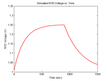
The resistance of the RTD is given by the equation $ R_{RTD} = R_o*(1 + \alpha \Delta T) $, where "α" is the temperature coefficient of resistance (TCR) for the RTD and $ R_o $ is the resistance at the reference temperature for the RTD. In the experimental apparatus, the RTD is hooked up as one element of a voltage divider with a pull-up resistor, R. The power supply input is 15 volts. Thus, the output voltage is: $ V_{RTD} = 15 * R_{RTD}/(R + R_{RTD}) $. The following code calculates RTD voltage measurements from sim1.temperature and stores the result in sim1.V_RTD, assuming $ R $ = 15kΩ, $ R_o $ = 1000Ω, $ \alpha $ = 3850 ppm/°C, and $ \Delta T $ is the difference, in Kelvin or Celsius, between the RTD reference temperature and the RTD temperature.
sim1.R_RTD_atZeroC = 1000;                                % Datasheet value of reference RTD resistance, Ω
sim1.RTDalpha = 3850;                                     % Datasheet value of RTD TCR, ppm/C
sim1.R_RTD = sim1.R_RTD_atZeroC ...
    * (1 + sim1.RTDalpha*1e-6 * (sim1.temperature-273));  % Compute RTD resistance, Ohms
sim1.R_pullup = 15e3;                                     % Pull-up resistor in voltage divider, Ohms
sim1.V_input = 15;                                        % Input voltage of divider, V
sim1.V_RTD = sim1.V_input * sim1.R_RTD ...
    ./ (sim1.R_pullup + sim1.R_RTD);                      % RTD votlage drop, V

figure(4)
plot(sim1.time, sim1.V_RTD, 'r');
xlabel('Time (sec)');
ylabel('RTD Voltage (V)');
title('Simulated RTD Voltage vs. Time');
Simulate DNA fraction for this temperature profile
Use the DnaFraction function given above to calculate the simulated fluorescence using the combined heating and cooling temperature profile that you just calculated.
sim1.dsDnaFraction = DnaFraction(sim1.DnaConcentration, ...
    sim1.temperature, sim1.deltaS, sim1.deltaH);

figure(5)
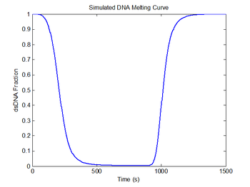
plot(sim1.time, sim1.dsDnaFraction);
title('Simulated DNA Melting Curve');
xlabel('Time (s)');
ylabel('dsDNA Fraction');

figure(6)
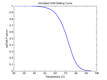
plot(sim1.temperature-273, sim1.dsDnaFraction);
title('Simulated DNA Melting Curve');
xlabel('Temperature (C)');
ylabel('dsDNA Fraction');
Issues experienced in practice
Now that you are confident that your fitting routine functions properly, you are ready to add sources of noise and other issues that you will experience in practice. It will be instructive for you to again try fitting a model to this "noisy" simulated data and discover how much the noise and bleaching affect your ability to estimate the true DNA melting curve.
Add some noise to the RTD signal
You will certainly notice noise on the signals you capture in the lab. Noise will be an extremely important (and annoying) factor in this experiment because the melting curves will be differentiated. Differentiation emphasizes noise. In order to ensure that your data analysis script effectively handles the noise you are likely to observe, simulated random and impulse noise will be added to the signals.
To simulate noise, we can use Matlab's randn function, which generates normally distributed random numbers with unity standard deviation. The two arguments tell randn to create a vector of random samples with size 1xlength(V_RTD).
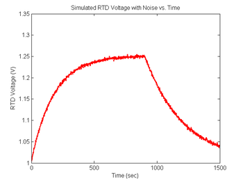
noise = 0.001 * randn(1,length(sim1.V_RTD))';    % Create noise vector, standard deviation=1mV
sim1.V_RTD = sim1.V_RTD + noise;                % Add simulated noise to the voltage signal

figure(8)
plot(sim1.time, sim1.V_RTD, 'r');
xlabel('Time (sec)');
ylabel('RTD Voltage (V)');
title('Simulated RTD Voltage with Noise vs. Time');
Revisit your code from DNA Melting: Simulating DNA Melting - Basics and using the approach above add noise to your RTD voltage signal, then explore the behavior of your code for different levels of noise. In particular, you can add differentiation of the curve from Figure 6 and discover the issues with attempts to differentiate that signal without additional processing. You will likely find that you first need to either sort or bin your temperature data so that the f vs T function can be differentiated. Then also run this data through your fit function and observe any difference in the fit statistics.
You are also encouraged to add noise at additional frequencies that you think might be present in the lab, then attempt to filter that data in Matlab to test the effectiveness of the RTD voltage filter design that you built in the lab. To do this, generate the noise (perhaps 60 Hz, pink noise, possibly high frequency noise from switching in the overhead lights, or even noise on the earth ground that could be coming from equipment elsewhere in the building) and add it to the signal from Figure 8. Remember it is a long way to the earth from our lab. Next filter that signal using your transfer function and the matlab command lsim. Then again run this data through your fit function.
Add some noise to the sample fluorescence signal
Maybe too much impulse noise at present
Now that we have added noise to the RTD voltage signal, the next step is to do the same for the fluorescence signal.
The output range of the transimpedance amplifier depends on many factors, including: dsDNA quantity, illumination intensity, fluorophore efficiency, optical system gain, photodiode efficiency, and electronic amplifier gain. All of the factors except dsDNA concentration essentialy remain constant. Thus, the output of the transimpedance amplifier can be modeled by a single overall system gain factor times the dsDNA fraction. In addition, the amplifier output may be offset by a constant DC value, which is simple to model. (If the output of your apparatus drifts significantly over time, you will need to improve your implementation and methods to minimize this.)
The output range of the transimpedance amplifier over the course of an experimental run can vary depending on several factors, including the amplifier gain, optical system gain, etc... A typical setup might produce values between, say, 0.5 and 7.2 Volts. The simulation code generates two random numbers to set the range and minimum value of the data. Your data analysis script will have to normalize the amplifier output voltage to a fractional value between 0 and 1. (What assumptions will you make about dsDNA concentration to do the normalization?)
In addition to white Gaussian noise, shot noise from the photo diode and Johnson noise in your feedback resistors, the high gain amplifier sometimes produces impulse noise. This can be caused by small static discharges, for example when a charged person sits down in a chair in the lab, or by machinery switching on or off somewhere else in the building. Each of these latter noise sources would generally show up on your ground reference, even when connected to the building earth ground, an often imperfect grounding source. Your goal is first to provide as much filtering as possible in your circuitry. However, these noise sources are difficult to completely eliminate, so it is a good idea to include some filtering in your data analysis script.
Range = 5 + 4 * rand();                              % Range between 5 and 9
Minimum = 2 * rand() - 1;                            % Minimum between +/- 1
sim1.V_f = Range * sim1.dsDnaFraction + Minimum;     % Scale output
noise = 0.01 * randn(1,length(sim1.V_f))';           % Random noise, standard deviation=10mV
sim1.V_f = sim1.V_f + noise;                         % Add random noise

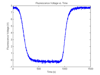
figure(9)
plot(sim1.time, sim1.V_fNoisy)
title('Fluorescence Voltage vs. Time');
xlabel('Time (s)');
ylabel('Fluorescence Voltage (V)');
As in the last section, revisit your code from DNA Melting: Simulating DNA Melting - Basics but this time add noise to your fluorescence voltage signal, then explore the behavior of your code for different levels of noise. Then again run this data through your fit function.
Here too you are encouraged to add noise at additional frequencies that you think might be present in the lab. What could you do to minimize the effects of these noise sources? Think of solutions both at the hardware level and at the software level and model both of them.

