20.309: Biological Instrumentation and Measurement
Assignment details
This assignment has 2 parts:
- Part 1: Use the epifluorescence microscope you built to image fixed biological samples, and use the flat-field correction code you wrote for Assignment 2 to address non-uniform illumination;
- Part 2: Explore interesting calculations and considerations to guide your experimental design with fluorescence.
Submit your work on Stellar in a single PDF file with the naming convention <Lastname><Firstname>Assignment3.pdf. Here is a checklist of all things you have to turn in:

|
Here is a comprehensive list of what you need to turn in:
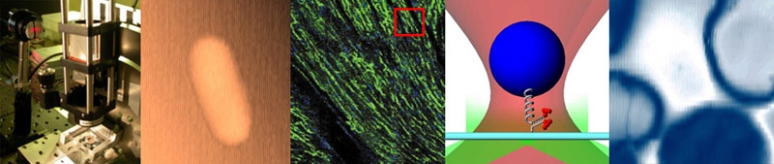
- A figure with images of the 3.26 μm fluorescent microsphere samples, and the stained cell samples with and without Cyto-D.
- For each sample, create 1 figure with 5 panels.
- The panels of the figure should be: A) unprocessed image; B) reference image; C) dark image; D) flat-field corrected image; and E) histogram.
- In the caption, specify the exposure and gain settings. Each image should have a scale bar. State the dimension of the scale bar in the caption.
- For panel E, plot histograms of the unprocessed, dark, reference, and corrected image on the same set of axes. Plot log10( count ) on the vertical axis and intensity on the horizontal axis. Use a line plot instead of a bar chart for the histogram.
- Image profile
- For one reference, dark and cell image set, plot an intensity profile across the same diagonal. You may also use a bead image, along with it's unique reference and dark images. The intensity of your three images should be on the same scale, i.e., 0 to 65,535 or 0 to 1. Place all three profiles on a single set of axes for comparison. (Use the improfile command in MATLAB.)
- Discussion
- How did your beam expander design affect your images?
- What differences did you observe between the cells with and without CytoD?
- Answers to all questions in Assignment 3, Part 2.
|
Navigation
Back to 20.309 Main Page
Background reading
