20.109(F21):M2D7
Contents
Introduction
In the previous laboratory sessions you performed a BLI assay to test 'hits' that were identified using SMM in an effort to study the interaction of these compounds with our protein of interest, PF3D7_20109-F21. Today you will complete the analysis and interpretation for the data you collected.
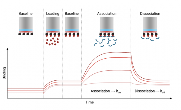
Recall that the BLI assay is able to measure the kinetics of binding between the protein of interest and the small molecule compounds. The values acquired from the BLI assay allow you to define the $ K_D $ which can give insight to the likelihood of the compound actually working as a drug against the protein target. The steps in the exercise for today will help you analyze the data and interpret the results.

Protocols
Part 1: Analysis of BLI data for small molecule binding to target protein
In this experiment, you used biolayer interferometry (BLI) to measure the binding kinetics of several small molecules to your target protein. We have conceptually explored the analytical framework that allows determination of the association and dissociation rate constants, and the equilibrium dissociation constants. Please refer to the handout from the previous class to review this information!
Here, you will step through some aspects of this analysis using experimental data you collected as a class, and interpret the results to share some insights on how well the various control, and test compounds interact with the target protein.
You can access your binding data by group, the class data by compound, and idealized data in this Dropbox folder BLI data
There are a series of guiding questions, the answers to which should inform your thought process in approaching the Results and Discussion sections of your research paper.
Protein binding
A key step in the BLI experiment is successful and stable immobilization of the target protein to the sensor probe.
- Examine your data and provide an illustration of the protein loading step. Describe whether protein immobilization has occurred successfully. Explain your reasoning.
- Ideally, your protein will remain tightly associated with the sensor probe over the entire duration of the experiment. Why is this important?
- Examine your datasets and describe whether stable protein association with the probe has been achieved. Include an illustration from your collected data to support your reasoning.
Reference sensor
In our experiment, we wish to observe and analyze the binding of compound to the immobilized protein specifically rather than to the sensor probe.
- How was this accomplished in your experiment?
- For your group’s positive and negative control and test compound dataset, how significant a problem is background binding to the probe across the various concentrations tested? Provide a succinct, quantitatively reasoned basis for your assessment.
Small molecule binding
Compound association and dissociation phases occurred at various intervals during the experiment at different compound concentrations. In a pre-analysis step, the association and dissociation response traces for each tested compound concentration has been aligned to facilitate plotting compound binding and dissociation from the protein-bound* and reference probes on the same x-axis (time). These data can be found in the relevant compound folder with filename “02_Processed without subtraction”.
Important note: Signal due to loading protein onto the probe has already been subtracted.
- For your group’s positive and negative controls and assigned test compound data set, perform the data analysis step that will allow you to detect specific binding of compound (if any) to the immobilized protein.
- Make Response versus time plots for each compound separately, but with the various concentrations overlaid. Qualitatively assess these plots (e.g., for which can you observe distinct association and dissociation phases, and how do these properties change with varying compound concentrations; are there discernible trends; comment specifically on which plots might you expect to be able to extract potentially meaningful quantitative analyses).
Analysis of fitted data
For this experiment, we have assumed that 1:1 protein: small molecule binding stoichiometry is the relevant analytical model. For each compound across the various tested concentrations, we have provided a file (“03_Processed Subtracted FIt global 1to1”) containing background-subtracted Response versus time data along with the “fitted” plot arising from a global fit to the 1:1 model.
Important note: In a ‘global fit’, the response versus time data obtained across the various compound concentrations are simultaneously considered to derive a single set of fitted parameters that best describe the data collectively. In contrast, a ‘local fit’ uses data from each compound concentration separately to derive the best fit to that single response versus time curve.
- For your group’s positive and negative controls and test compound, confirm that the response versus time plots you derived in question 2 in the last section match the corresponding plots of the experimental data in the relevant “03_Processed Subtracted FIt global 1to1” file.
- For the Class’ Positive Control 1 and Positive Control 2 data, plot the experimental and globally fitted data for each tested concentration overlaid on the same plot. Qualitatively, how well do the experimental and fitted data agree? Are some fits better or worse, and are there discernible patterns? What are potential key reason(s) driving differences between the experimental and fitted curves?
- We have also provided ‘local fit’ Class’ Positive Control 1 and Positive Control 2 data (“03a_Processed Subtracted Fit local 1to1”). Qualitatively, how well do the experimental and fitted data agree? Are some fits better or worse, and are there discernible patterns? Does global or local fitting result in qualitatively better fitted curves? Why might this occur?
- We have also provided modified ‘partial global fit’ class’ Positive Control 1 and Positive Control 2 data (“03b_Processed Subtracted Fit global 1to1-mod”). Plot these and comment qualitatively on the level of agreement between the experimental and fitted data. Describe what has changed in this analysis, and how this is influencing the outcome.
- Now examine the values assigned to the various parameters during the fitting performed in step 2 above (“04_kineticanalysistableresults1to1global”), step 3 above(“04a_kineticanalysistableresults1to1local”) and step 4 above (“04b_kineticanalysistableresults1to1global-mod”).
Part 2: Interpretation of BLI results
- Focus your attention on the following key parameters for your detailed analysis: kd, kobs, ka, KD, Req, and Rmax. Note these all have associated standard deviations (SD) and the linear regression analysis returns an R2 fitting statistic (2 degrees of freedom) describing how well the fitted model predicts the experimental data.
- Use a combination of your qualitative analysis and the fitting statistics to provide a clear and succinct justification for choosing to further interpret the data as analyzed in either 4b, 4c or 4d. Include any concerns you have about the chosen analysis (for e.g., confidence in any of the fitted values, etc.).
- As compound concentration is varied, which fitted parameters do you expect to change based on the assumed 1:1 analytical model? Make representative plots to summarize the observed trends in these parameters as a function of tested concentration. Compare the trends for Positive Control 1 and Positive Control 2. What are possible reasons for your observation(s), and what would you expect if we could further increase compound concentration?
- Compare the equilibrium binding constant for Positive Control 1 and Positive Control 2. Does one bind to the protein with higher apparent affinity? Interpret the rate constants (ka, kd) to rationalize how the higher affinity is attained.
- We have also provided an Instructor generated data set for Positive Control 1. Plot the overlaid experimental and global fit data provided. Compare these plots qualitatively as well as based on the quantitative outputs (global or local, depending on your analysis in e above). How do the binding parameters compare between the Class- versus Instructor-collected data? How would you use this additional information to benchmark your results?
- For the test compound assigned to your group, comment on the plots generated in 2b/ 3a.
- Can you observe binding of your compound to the target protein at all/ some/ none of the concentrations tested?
- A global 1:1 fit of the data and the resulting fitted parameters have been provided. Examine the plots of your overlaid experimental and fitted data. Both qualitatively and quantitatively, how well does the model fit the data?
- Is it meaningful/ appropriate to globally fit the experimental data for your test compound? Explain your reasoning.
- By visually inspecting your data, is there an analysis that could give you some quantitative insight? What would be some limitations associated with your proposed approach?
- We have collated data for all 4 test compounds from across the lab groups, and performed local fit analyses. For each compound, data for 1-2 tested concentrations showed some discernible association and dissociation.
- Apply as much of the analysis presented in 4e (i-iii) above as relevant. Compare how well these test compounds bind to the protein relative to Positive Control 1 and Positive Control 2.
- How confident are you in the calculated parameters and why? How does this limit or facilitate analyses comparing relative binding?
- Some additional questions to consider:
- What are some factors limiting use of the BLI approach to determine binding of small molecules to immobilized protein targets? How would these manifest experimentally and impact downstream analysis?
- How might a protein in solution that putatively binds a compound immobilized on an SMM be found not to interact when the protein is immobilized on a probe and the small molecule presented in solution phase?
- What does high binding affinity tell us about the molecular/ atomic-level interactions of a small molecule with a protein target?
- Does BLI let us know directly whether two different molecules share the same binding site on a target protein?
