Difference between revisions of "Assignment 9, Part 3: Fitting your data"
Juliesutton (Talk | contribs) (Created page with "Congratulations! you should now have a working version of your analysis code. ==Estimate model parameters for real data== Use your model function and nlinfit to estimate the ...") |
(→Residual plot) |
||
| (13 intermediate revisions by 3 users not shown) | |||
| Line 1: | Line 1: | ||
| + | __NOTOC__ | ||
Congratulations! you should now have a working version of your analysis code. | Congratulations! you should now have a working version of your analysis code. | ||
==Estimate model parameters for real data== | ==Estimate model parameters for real data== | ||
| − | Use your | + | Use your newly developed code to estimate the parameters associated with a set of DNA melting data that you took using your instrument. (You may use a data set you took from a previous week.) |
| + | |||
| + | ''Tip:'' you will be running this type of operation many times for many different DNA melting curves in the next couple weeks. It may be helpful to write a function to make this task easily repeatable. | ||
{{Template:Assignment Turn In|message = <br/> | {{Template:Assignment Turn In|message = <br/> | ||
| − | #Plot your fluorescence data as a function of temperature, your model function with initial guesses, and your model function with best fit parameters on the same set of axes. | + | #Plot your fluorescence data as a function of block temperature, your model function with initial guesses, and your model function with best fit parameters on the same set of axes. |
| − | #Record your estimates for &Delta H and &Delta S | + | #Record your estimates for ΔH and ΔS. Calculate T<sub>m</sub>. |
#How do these thermodynamic parameters compare to the predicted values you obtained from DINAmelt or OligoCalc? | #How do these thermodynamic parameters compare to the predicted values you obtained from DINAmelt or OligoCalc? | ||
}} | }} | ||
| − | == | + | ==Residual plot== |
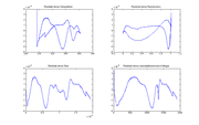
| − | + | [[Image:Residual plot for DNA data.png|thumb|right|Residuals plotted versus time, temperature, fluorescence, and the cumulative sum of fluorescence]] | |
| + | Observed values differ from predicted values because of noise and systematic errors in the model. Residuals are the difference between experimental observations and model predictions, ''V<sub>f,measured</sub>''−''V<sub>f,model</sub>''. Ideally, the residuals should be random and identically distributed. | ||
| − | The | + | The plots at right show ''V<sub>f,measured</sub>''−''V<sub>f,model</sub>'', versus temperature, time, fluorescence, and the cumulative sum of fluorescence. The residuals are clearly not random and identically distributed. This suggests that the model does not perfectly explain the observations. The scale of the plot is much smaller than the data plot — about one percent of the data scale. |
| − | + | A perfect model might require dozens of added parameters and additional physical measurements. | |
| − | + | ||
| − | + | ||
| − | + | ||
| − | + | ||
| − | + | ||
| − | + | ||
| − | + | Plotting the residuals versus different variables can help suggest what factors are not modeled well. | |
| − | + | ||
| − | + | {{Template:Assignment Turn In|message= Plot the residuals vs. | |
| − | + | # time, | |
| − | + | # temperature, and | |
| + | # fluorescence. | ||
| + | }} | ||
| − | [[Image: | + | ==Finding double stranded DNA fraction from raw data== |
| − | + | [[Image:Corrected DNA data.png|thumb|right]] | |
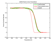
| − | + | The inverse function of the melting model with respect to ''V<sub>f,measured</sub>''(''t'') is helpful to visualize discrepancies between the model and experimental data caused by random noise in ''V<sub>f,measured</sub>'' and systematic error in the model ''V<sub>f,model''. The function, | |
| + | |||
| + | ::<math>C_{ds,inverse-model}(V_{f,measured}(t)) = \frac{V_{f,measured}(t) - K_{offset}} {K_{gain} S(t) Q(t)}</math>, | ||
| + | |||
| + | is itself a model. This model estimates the concentration of double stranded DNA based on the observations <math>V_{f,measured}(t)</math> and the models for bleaching and quenching. | ||
| + | |||
| + | The estimated melting curve may be directly compared with simulations, measurements or other predictions of the true melting curve. The plot at right shows an example of ''C<sub>ds,inverse-model</sub>''(''t'') versus ''T<sub>sample</sub>''(''t''). The estimated melting curve is shifted to the right compared to the simulated melting curve, possibly due to systematic error in the sample temperature model. The estimated melting curve also serves as a comparison to the thermodynamic model developed in [[DNA Melting Thermodynamics]], or to any other independent measurement or model of the melting curve, i.e., the concentration of dsDNA vs sample temperature. | ||
| + | |||
| + | {{Template:Assignment Turn In|message= Write a function to convert fluorescence into fraction of double stranded DNA. For at least one experimental trial, plot <math>\text{DnaFraction}_{inverse-model}</math> versus the ''sample temperature'' <math>T_{sample}</math> ([http://measurebiology.org/wiki/File:Inverse_cuvrve.png example plot]). On the same set of axes plot DnaFraction versus <math>T_{sample}</math> using the best-fit values of ΔH and ΔS. Finally, plot simulated dsDNA fraction vs. temperature using data from DINAmelt or another melting curve simulator.}} | ||
| + | |||
| + | ==Comparing the known and unknown samples== | ||
| + | In the next assignment, you will be comparing an unknown sample to a set of three known samples in order to determine its identity. Read through this page: [[Identifying the unknown DNA sample]], to learn about the statistics behind making multiple comparisons. | ||
{{Template:Assignment Turn In|message=<br/> | {{Template:Assignment Turn In|message=<br/> | ||
| − | + | Explain the statistical method you will use to identify your group's unknown sample in Assignment 10. | |
| − | + | * State the acceptance/rejection criteria for any hypotheses/tests you will use. | |
| − | + | * This page may be a helpful reference: [[Identifying the unknown DNA sample]]. | |
}} | }} | ||
{{Template:Assignment Turn In|message = Append all of the code you wrote for Parts 1, 2 and 3 of this assignment. }} | {{Template:Assignment Turn In|message = Append all of the code you wrote for Parts 1, 2 and 3 of this assignment. }} | ||
| + | |||
| + | {{Template:Assignment 9 navigation}} | ||
Latest revision as of 22:39, 27 April 2018
Congratulations! you should now have a working version of your analysis code.
Estimate model parameters for real data
Use your newly developed code to estimate the parameters associated with a set of DNA melting data that you took using your instrument. (You may use a data set you took from a previous week.)
Tip: you will be running this type of operation many times for many different DNA melting curves in the next couple weeks. It may be helpful to write a function to make this task easily repeatable.
Residual plot
Observed values differ from predicted values because of noise and systematic errors in the model. Residuals are the difference between experimental observations and model predictions, Vf,measured−Vf,model. Ideally, the residuals should be random and identically distributed.
The plots at right show Vf,measured−Vf,model, versus temperature, time, fluorescence, and the cumulative sum of fluorescence. The residuals are clearly not random and identically distributed. This suggests that the model does not perfectly explain the observations. The scale of the plot is much smaller than the data plot — about one percent of the data scale.
A perfect model might require dozens of added parameters and additional physical measurements.
Plotting the residuals versus different variables can help suggest what factors are not modeled well.
| |
Plot the residuals vs.
|
Finding double stranded DNA fraction from raw data
The inverse function of the melting model with respect to Vf,measured(t) is helpful to visualize discrepancies between the model and experimental data caused by random noise in Vf,measured and systematic error in the model Vf,model. The function,
- $ C_{ds,inverse-model}(V_{f,measured}(t)) = \frac{V_{f,measured}(t) - K_{offset}} {K_{gain} S(t) Q(t)} $,
is itself a model. This model estimates the concentration of double stranded DNA based on the observations $ V_{f,measured}(t) $ and the models for bleaching and quenching.
The estimated melting curve may be directly compared with simulations, measurements or other predictions of the true melting curve. The plot at right shows an example of Cds,inverse-model(t) versus Tsample(t). The estimated melting curve is shifted to the right compared to the simulated melting curve, possibly due to systematic error in the sample temperature model. The estimated melting curve also serves as a comparison to the thermodynamic model developed in DNA Melting Thermodynamics, or to any other independent measurement or model of the melting curve, i.e., the concentration of dsDNA vs sample temperature.
| |
Write a function to convert fluorescence into fraction of double stranded DNA. For at least one experimental trial, plot $ \text{DnaFraction}_{inverse-model} $ versus the sample temperature $ T_{sample} $ (example plot). On the same set of axes plot DnaFraction versus $ T_{sample} $ using the best-fit values of ΔH and ΔS. Finally, plot simulated dsDNA fraction vs. temperature using data from DINAmelt or another melting curve simulator. |
Comparing the known and unknown samples
In the next assignment, you will be comparing an unknown sample to a set of three known samples in order to determine its identity. Read through this page: Identifying the unknown DNA sample, to learn about the statistics behind making multiple comparisons.
| |
|
| |
Append all of the code you wrote for Parts 1, 2 and 3 of this assignment. |
- Assignment 9 Overview
- Part 1: model function
- Part 2: test your code with simulated data
- Part 3: fitting your data
Back to 20.309 Main Page

