Difference between revisions of "20.109(S16):Flow cytometry and paper discussion (Day7)"
Noreen Lyell (Talk | contribs) (→Part 2: Analyze flow cytometry data) |
Noreen Lyell (Talk | contribs) (→Part 2: Analyze flow cytometry data) |
||
| Line 71: | Line 71: | ||
#*Enter the median values from the sample spreadsheet to test your template. | #*Enter the median values from the sample spreadsheet to test your template. | ||
#[[Image:Sp16 M2D7 plot statistics.png|thumb|right|500px|'''Flow cytometry plot statistics summary.''']]Now let's look at the data collected using your conditions. | #[[Image:Sp16 M2D7 plot statistics.png|thumb|right|500px|'''Flow cytometry plot statistics summary.''']]Now let's look at the data collected using your conditions. | ||
| − | #*Open the pdf posted to the M2D7 Discussion page named "Instructor FC plots" and the sample key named "Instructor FC sample key" and find the plot for sample #5 (M059K cells co-transfected with pMAX_mCherry and pMAX_EGFP). | + | #*Open the pdf posted to the M2D7 Discussion page named "Instructor FC plots" and the sample key named "Instructor FC sample key" and find the plot for sample #5 (M059K cells co-transfected with pMAX_mCherry and pMAX_EGFP). At the bottom of the page you should see a table similar to the one shown at the right. |
| + | #*The values in this table are the counts that were measured for this sample. Consider the following: | ||
| + | #**#Events = the number of cells counted based on the gate established (i.e. the number of red cells is based on the mCherry gate) | ||
| + | #**%Parent = the percentage of cells in a given population (i.e. the number of red cells within the live cell population) | ||
| + | #**FITC-A = filter used to 'see' green cells | ||
| + | #**PE-Cy5-5... = filter used to 'see' red cells | ||
#After you understand the instructor data, skim over your 12 sample plots. Can you see apparent differences between K1, K1+inhibitor, and xrs6? | #After you understand the instructor data, skim over your 12 sample plots. Can you see apparent differences between K1, K1+inhibitor, and xrs6? | ||
Revision as of 17:04, 2 April 2016

Contents
Introduction
We hope that you’ll leave lab today with a sense of accomplishment, after inspecting your raw flow cytometry data and then calculating NHEJ repair values. Unfortunately or excitingly – depending on your perspective – it turns out in scientific research that the hard work is just beginning once the data is quantified! Interpreting the data and drawing (sometimes tentative) conclusions requires deep reading and thinking – a process that shouldn’t be rushed.
Now is the time to clearly understand the nature of the flow cytometry controls that you will examine. For each cell population, you prepared two DNA mixtures: (A) intact pMAX_mCherry plus intact pMAX_EGFP, and (B) intact pMAX_mCherry plus damaged pMAX_EGFP_MCS. The re-circularization of pMAX_EGFP_MCS (minus the nonsense insert) will be our most direct readout of how much repair occurred. In this simplest view, broken DNA = no fluorescent signal, and repaired DNA = green fluorescent signal. However, it is important to consider the possibility that one cell population simply took up more plasmid DNA than another. In more technical terms, what if the transfection efficiency is higher for one cell type than for the other, and therefore the repair rate artificially appears higher? To control for this we co-transfected with intact pMAX_mCherry, which serves as a transfection control. Using the transfection control data, we will normalize for differences in DNA uptake. It is also important to think about the uptake of pMAX_mCherry compared to the uptake of pMAX_EGFP_MCS. What if the plasmids are taken up at different frequencies, or successfully expressed at different frequencies and/or signal intensities? Here is where the dual intact control is useful. It shows us the typical ratio of mCherry:EGFP uptake and expression, which we can use as a secondary normalization. Note that we use pMAX_EGFP as a control rather than pMAX_EGFP_MCS, because the latter will have very low expression that is not representative of the repaired construct: the nonsense insert separates the promoter and gene by too great a distance for robust expression.
Putting all of the above information together, the NHEJ repair frequency equation can be determined in three steps:
- (1) Raw F reporter expression = % cells positive for F x MFI(F) = "RAW"
- F can be "mCherry" or "EGFP" in our case
- MFI is mean fluorescence intensity or median fluorescence intensity
- (2) Normalized EGFP expression $ \qquad ={RAW_{EGFP} \over RAW_{mCherry}}\qquad $ = "NORM"
- (3) Reporter expression percent $ \qquad ={NORM_{EGFP.damaged} \over NORM_{EGFP.intact}}\qquad $ = NHEJ repair value
First, reporter expression for mCherry and EGFP alike will be calculated by multiplying percentage of positive cells by fluorescence intensity (FI). We have a choice of whether to use mean, geometric mean, or median fluorescence intensity. Median fluorescence is least susceptible to being influenced by a few outliers, while geometric mean is generally more appropriate for log scale data than arithmetic mean. For normally distributed populations, all three values should be pretty similar. In practice, we have found that while mean and median FI are very different values, after normalization the ultimate NHEJ repair values are quite similar, so we will use the mean value.
The second step is to calculate the ratio of EGFP to mCherry reporter expression for each sample. The final step is to divide the damaged-EGFP:mCherry ratio by the maximal possible “repair,” namely the intact-EGFP:mCherry ratio. Convince yourself that this parameter essentially provides the fraction of pMAX_EGFP_MCS repaired.
Most of your time today will be spent at the computer, quantifying your flow cytometry data. Use this time to get a strong start on the data analysis for your Systems engineering research article. On M2D9, we will use statistics to further analyze our data.
Protocols
Part 1: Paper discussion
We will start today with a discussion of the Dietlein et al. research article. In their research, the authors completed a screen to examine 1319 cancer-associated genes from 67 cell lines to identify cancer-cell specific mutations that are associated with DNA-PKcs dependence or addiction. A paradox exists in cancer as whole genome sequencing has revealed that the cells of many tumor types have mutations in genes necessary for DNA repair. These mutations are responsible for cells becoming cancerous, but are also detrimental because, just like normal cells, cancer cells must divide to survive. Thus, a cancer cell will develop an ‘addiction’ to a DNA repair pathway – specifically, a pathway different from the one with the mutation that caused the cell to generate a tumor. Recent cancer therapies seek to exploit this addiction by targeting the intact pathway used by the tumor cells to repair DNA damage due to intrinsic breaks that occur during replication. In addition, the effectiveness DNA damage induced by chemotherapy treatment may be enhanced by also disrupting the functional repair pathways of tumor cells. The review article by Shaheen et al. provides further information on repair pathway addiction as a target in cancer treatment.
Our paper discussion will be guided by all that you have learned about how to write a cohesive story that clearly reports the data and provides strong support for the conclusions made about the data. During the paper discussion, everyone is expected to participate - either by volunteering or by being called upon!
Introduction
Remember the key components of an introduction:
- What is the big picture?
- Is the importance of this research clear?
- Are you provided with the information you need to understand the research?
- Do the authors include a preview of the key results?
Results
Carefully examine the figures. First, read the captions and use the information to 'interpret' the data presented within the image. Second, read the text within the results section that describes the figure.
- Do you agree with the conclusion(s) reached by the authors?
- What controls are included and are they appropriate for the experiment performed?
- Are you convinced that the data are accurate and/or representative?
Discussion
Consider the following components of a discussion:
- Are the results summarized?
- Did the authors 'tie' the data together into a cohesive and well-interpreted story?
- Do the authors overreach when interpreting the data?
- Are the data linked back to the big picture from the introduction?
Part 2: Analyze flow cytometry data
In the previous laboratory session, you learned how the gates are established in flow cytometry. This very important step is necessary in enabling you to distinguish and count the specific cell populations within your samples. Today you will analyze the numerical data, or counts, that were collected for your transfection conditions based on the mCherry and EGFP gates.
Before you calculate the frequency of DNA repair that occurred in your samples, examine the data obtained in Spring 2015 to acquaint yourself with calculations discussed in prelab. The spreadsheet below shows a template used to calculate the NHEJ repair efficiency using the EGFP:BFP reporter system employed by students previous to this semester. Use the data in the spreadsheet to answer the questions below.

- To test yourself, use the numbers provided in the sample spreadsheet to calculate the NHEJ efficiency with the median fluorescent values by hand.
- Include your math in your notebook.
- Now create a template in Excel that will enable to quickly determine the values for your samples.
- Feel free to use the format of the sample NHEJ calculator.
- Enter the median values from the sample spreadsheet to test your template.
- Now let's look at the data collected using your conditions.
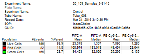 Flow cytometry plot statistics summary.
- Open the pdf posted to the M2D7 Discussion page named "Instructor FC plots" and the sample key named "Instructor FC sample key" and find the plot for sample #5 (M059K cells co-transfected with pMAX_mCherry and pMAX_EGFP). At the bottom of the page you should see a table similar to the one shown at the right.
- The values in this table are the counts that were measured for this sample. Consider the following:
- Events = the number of cells counted based on the gate established (i.e. the number of red cells is based on the mCherry gate)
- %Parent = the percentage of cells in a given population (i.e. the number of red cells within the live cell population)
- FITC-A = filter used to 'see' green cells
- PE-Cy5-5... = filter used to 'see' red cells

- After you understand the instructor data, skim over your 12 sample plots. Can you see apparent differences between K1, K1+inhibitor, and xrs6?
- Now that you have a good conceptual understanding of the data, it's time to crunch some numbers. Open the .csv file and save it as a newly named .xlsx file.
- Begin by deleting all of the rows except the twelve containing your own dataset.
- Next delete all of the columns except the few that interest you. Keep in mind that you need to know Green cell and Blue cell gating as a % of the parent gate, Live Cells. Class-wide, you are only required to do your calculations based on mean fluorescence intensity (MFI), but you should also keep the median data in case others want to use it.
- We recommend that you prepare a new Excel file with your NHEJ equations, and just copy-paste in the appropriate % and MFI data; this approach is a versatile one. Your final worksheet might look similar to the screenshot below.
- Remember that for each of the twelve wells you should calculate raw reporter expressions and a BFP/GFP normalized value. Then, for each intact/cut pair you can calculate an NHEJ value. In this way, we should have quadruplicate NHEJ values for most repair topology/cell population conditions, which will allow us to do statistical comparisons.
Reference information:
| Day | Tube # | Condition |
|---|---|---|
| T/R | 1 | Mock transfection |
| T/R | 2 | GFP Intact Only |
| T/R | 3 | BFP Intact Only |
| W/F | 1 | Mock transfection |
| W/F | 2 | GFP Intact Only |
| W/F | 3 | BFP Intact Only |
You must email your Excel sheet to Shannon (T/R) or Leslie (W/F) before leaving lab today. We instructors will post a summary file for ease of class-wide data analysis by Wednesday evening or Thursday morning.
Next day: Journal Club II
Previous day: DNA repair assays