20.109(S24):M2D7

Introduction

TEM from NanoScience Instruments

The Transmission Electron Microscope (TEM) achieves its remarkable resolution by 'illuminating' samples using an electron beam in a vacuum rather than using a conventional light source in air. TEM enables 0.14 nm resolution. At this resolution, one can distinguish individual planes of atoms – making TEM an excellent materials characterization instrument. The visualization of single atoms allows one to determine many parameters that describe the structure of the material, such as crystal plane spacing. Additionally, TEMs can be equipped to perform energy-dispersive X-ray spectroscopy analysis (EDX/EDS/XEDS) or electron energy-loss spectroscopy analysis (EELS). The former, EDX, enables identification of the atomic composition of heavier elements in the material. EDX has limited detection of elements below sodium (Na) on the periodic table and no detection of elements below carbon (C). The latter, EELS, is most sensitive to lighter elements, typically from carbon to the 3d transition metals. EELS can reveal atomic composition, electronic properties of the valence and conduction band of a material, surface properties, and chemical bonding.

Although we will be using TEM for materials characterization, it should also be noted that TEM is used for the analysis of biological materials as well. Since the electron beam passes through the sample that is being examined, the sample must be sufficiently thin and sufficiently sturdy to be hit by electrons in a vacuum. Rather than imaging single atoms, biological samples display contrast of components via different densities. Areas of higher density show up as a darker color than areas of low density, creating a "shadow image." It is important to remember that many biological materials are damaged or destroyed by the incoming electrons and that the TEM can image only the species that survive this harsh treatment.

In TEM, the denser parts of the sample will absorb or scatter some of the electron beam, and it's the scattered electrons or those that pass through the sample that are focused using an electromagnetic lens. This "electron shadow" then strikes a fluorescent screen, giving rise to an image that varies in darkness according to the sample's density. For samples that are amenable to TEM, this form of examination can allow observation of ångström-sized objects and of cellular details down to near atomic levels.

The principles behind transmission electron microscopy are analogous to the principles behind an optical microscope. Instead of light and glass lenses, however, the TEM utilizes an electron beam focused via electromagnetic lenses. Since the TEM utilizes an electron beam rather than visible light, the microscope must also function under a vacuum. This condition allows the electrons to remain traveling in a straight line because they have no air particles with which to collide.

Specifically, at the top of the column of a TEM, a high voltage electron beam is emitted by a cathode and focused via a condenser lens. Then the beam is transmitted through the specimen. The resulting image is then magnified through a series of electromagnetic lenses until it is recorded by a fluorescent screen or camera.

Protocols

Part 1: Examining TEM images of cadmium sulfide particles

TEM grid with carbon mesh, photographed at 60X magnification

We will be imaging our cadmium sulfide particles via TEM. To prepare for TEM, your previously collected samples were dotted onto a very thin TEM grid.

• TEM grids can be made of many kinds of materials. Each design, however, includes lines of a conductive metal which disperses the electron beam and thereby prevents destruction of the sample from the harsh beam.
• Our TEM grids are composed of a nickel mesh with carbon mesh strung between the grids.

To prepare grids to image cadmium sulfide particles, the following steps were performed in the Belcher lab.

1. Sonicate yeast to dislodge cadmium sulfide particles from cell surface
2. Filter supernatent to remove remaining yeast debris.
3. Vortex the filtered supernatent for at least 1 minute and immediately remove 10 μL of the cadmium sulfide suspension to place on the TEM grid that you have balanced in the tension tweezers.
   

   

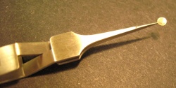   TEM grid balanced in tweezers
   
   
4. Allow the cadmium sulfide particles to settle onto the grid undisturbed for 10 minutes.
5. Remove the droplets of water from the grids by touching the edges with a Kimwipe, thereby wicking the solution off the grid.
6. Wash the grids by adding 10 μL of sterile water onto each grid.
7. Allow the grids to sit with water for 1-3 minutes and then wick dry.
8. Wash the grids by adding 10 μL of 100% EtOH onto each grid.
9. Allow the grids to sit with EtOH for 1-3 minutes and then wick dry, if it hasn't air dried.

1. Once a sample has been applied to our TEM grids, we will only visualize the portions of the sample contacting the carbon mesh, along with any imperfections in the carbon mesh itself.

Today you will image the TEM grids that contain these cadmium sulfide particles. Due to space limitations, only 2 groups can join Prof. Belcher and Dr. Jifa Qi for the imaging at a time. Please bring computers to work on the Research Article during your waiting time.

Part 2: Examining cadmium sulfide particles with fluorescence spectroscopy

You will also be using fluorescence spectroscopy to assess the fluorescent properties of the cadmium sulfide particles you have collected with your yeast display model system.

1. Vortex to resuspend yeast pellet from M2D5.
   • The yeast in this pellet were incubated with 100uM cadmium nitrate for 24 hours before being harvested through centrifugation.
   • The media from this experiment was filtered and analyzed via ICP-OES.
2. Remove 5ul of yeast suspension and dilute it in 2ml dionized water.
3. Sonicate sample for 3 minutes to break apart yeast and dislodge cadmium sulfide particles.
   • In your demonstration with Dr. Jifa Qi, you will only sonicate for 1 minute. This should be enough to see cadmium sulfide fluorescence
4. Filter your sample to remove yeast debris and collect cadmium sulfide in the supernatent.
5. Pipette 1ml of supernatent into a cuvette and read on the fluorimeter
   • In the full-scale analysis of your cadmium sulfide particle production, Dr. Qi used both a reusable quartz cuvette to measure lower wavelength excitation (250nm), and disposable plastic cuvette to measure emission at a longer wavelenth excitation (300-450nm). By using the quartz cuvette, he was able to avoid interference by the polymers present in plastic disposable cuvettes. However, both cuvettes types produced data for analysis.
   • For your demonstration, you will use disposable cuvettes and a longer wavelength excitation (300-450nm).
6. Working with Dr. Qi, adjust control parameters on the fluorimeter to allow for accurate capture and quantification of fluorescent emission.
   • excitation wavelength
   • fluorescence wavelength range
   • measurement duration
7. Once you have measured the fluorescence emission of your sample, you will be able to compare the emission peak of your cadmium sulfide particles to control samples to determine the efficacy of your capture system.

Part 3: Work on data analysis for Research Article

Flow Cytometry:
To assess the induction in your system as well as the labeling of the cell surface peptides, you will analyze flow cytometry data comparing uninduced and induced cell populations. Each data set is comprised of Alexafluor-488 intensity measured for 100,000 cells. To analyze the data, you will determine the mean intensity of the fluorescent signal of your population, so that you can make overall comparisons between induced and uninduced groups. You should do this for your data and the controls. For your peptide data, you will also graph a histogram to more fully characterize your population of cells. The raw fluorescent data has been binned so that histograms can be created more easily.

ICP-OES:
To assess how well your YSD cells removed cadmium from the media environment, look at the Sp24_Report of Results pdf in the dropbox linked on the Class Data page.

1. Examine the standard curves. Is cadmium concentration able to be accurately measured using these wavelengths?
2. Copy your concentration data (for both wavelengths) into Excel for later use. Use the replicates to calculate a mean concentration. You will graph the mean concentration (in ppm) for your data and use the replicates to generate error bars during statistical analysis (M2D8).
3. Also copy the data for control peptides (6xG and 2xGCC) as well as the EV control. These will analyzed in the same way to make statistical comparisons.

Fluorimetry:
To assess the fluorescent emission of the cadmium sulfide particles collected in your model, you will graph the corrected emission spectra measured by fluorimetry. In your data, you will see the wavelength column matched with a column labeled S1/R1. This is the corrected fluorescent signal intensity. The signal (S) is corrected at each wavelength to account for any background signal produced by the excitation lamp (R). This also corrects for the fact that the lamp doesn't produce a uniform illumination across all wavelengths. To analyze this data, you will graph the signal at each wavelength as a line graph. From there you can determine the peak emission wavelength and intensity (height of the graph). You should also graph the controls to make comparisons to your data.

Additionally, you will measure the width of the emission spectra by reporting the Full Width At Half Maximum (FWHM). Divide the maximum intensity by 2 and find the two wavelengths on either side of the peak wavelength that corresponds to this number. Calculate the width. If you are missing one of the sides, you may estimate the width by multiplying one side by 2.

TEM:

Cadmium Sulfide particles produced by Sun et al. 2020. ΔMet17 without YSD peptides were grown in CSM and incubated with cadmium nitrate

You will examine a representative set of TEM images to qualitatively assess the quality of your cadmium sulfide quantum dot production. You will be able to use scale bars to identify the rough size of your Cadmium sulfide particles and compare the size of your particles to those published by the Belcher lab in Sun et al. 2020 (see image at the right). What are your qualitative assessments of the cadmium sulfide particles produced by this model system?

Reagents

• Cuvettes (VWR)
• FluoroHub Fluorimeter (Horriba Scientific)
• 400-mesh nickel Formvar grids (EMS) for TEM
• JEOL2010F Electron Microscope

Navigation links

Next day: Complete data analysis and organize Research Article figures

Previous day: Quantify cadmium removal from media