20.109(F17):Examine sub-nuclear foci abundance to measure DNA damage (Day6)

Introduction

The ability to bind specific proteins using antibodies, or immunoglobulins, is critical in immuno-fluorescence labeling and Western blot analysis. Antibodies are typically 'raised' in mammalian hosts. Most commonly mice, rabbits, and goats are used, but antibodies can also be raised in sheep, chickens, rats, and even humans. The protein used to raise an antibody is called the antigen and the portion of the antigen that is recognized by an antibody is called the epitope. Some antibodies are monoclonal, or more appropriately “monospecific,” and recognize one epitope, while other antibodies, called polyclonal antibodies, are in fact antibody pools that recognize multiple epitopes. Antibodies can be raised not only to detect specific amino acid sequences, but also post-translational modifications and/or secondary structure. Therefore, antibodies can be used to distinguish between modified (for example, phosphorylated or glycoslyated proteins) and unmodified protein.

Monoclonal antibodies overcome many limitations of polyclonal pools in that they are specific to a particular epitope and can be produced in unlimited quantities. However, more time is required to establish these antibody-producing cells, called hybridomas, and it is a more expensive endeavor. In this process, normal antibody-producing B cells are fused with immortalized B cells, derived from myelomas, by chemical treatment with a limited efficiency. To select only heterogeneously fused cells, the cultures are maintained in medium in which myeloma cells alone cannot survive (often HAT medium). Normal B cells will naturally die over time with no intervention, so ultimately only the fused cells, called hybridomas, remain. A fused cell with two nuclei can be resolved into a stable cell line after mitosis.

Generating monoclonal antibodies.

To raise polyclonal antibodies, the antigen of interest is first purified and then injected into an animal. To elicit and enhance the animal’s immunogenic response, the antigen is often injected multiple times over several weeks in the presence of an immune-boosting compound called adjuvant. After some time, usually 4 to 8 weeks, samples of the animal’s blood are collected and the cellular fraction is removed by centrifugation. What is left, called the serum, can then be tested in the lab for the presence of specific antibodies. Even the very best antisera have no more than 10% of their antibodies directed against a particular antigen. The quality of any antiserum is judged by the purity (that it has few other antibodies), the specificity (that it recognizes the antigen and not other spurious proteins) and the concentration (sometimes called titer). Animals with strong responses to an antigen can be boosted with the antigen and then bled many times, so large volumes of antisera can be produced. However animals have limited life-spans and even the largest volumes of antiserum will eventually run out, requiring a new animal. The purity, specificity and titer of the new antiserum will likely differ from those of the first batch. High titer antisera against bacterial and viral proteins can be particularly precious since these antibodies are difficult to raise; most animals have seen these immunogens before and therefore don’t mount a major immune response when immunized. Antibodies against toxic proteins are also challenging to produce if they make the animals sick.

Generating polyclonal antibodies.

In your experiment, you will use a primary antibody to bind the γH2AX foci. Then a secondary antibody will be used that is specific to the conserved region of the primary antibody. The use of secondary antibodies allows researchers to tag the primary antibody. In our assay, the tag is a 488 nm fluorescent dye that will enable us to visualize double-strand breaks via microscopy. As a reminder, during the last laboratory session you treated cells with two concentrations of either H₂O₂ or MMS for the H2AX assay. Since then, the teaching faculty fixed all the wells with paraformaldehyde. Your task for today is to permeabilize the cells, which will enable the antibodies to enter the cells and bind γH2AX.

Protocols

Part 1: Complete antibody staining for H2AX assay

Immunofluorescence staining chamber

At this point in the assay sterility is no longer a concern and you will complete the following steps in the main laboratory at your bench.

1. Obtain your 12-well plates from the front bench.
2. Gather aliquots of 1 X TBS and 1% BSA in TBS from the front laboratory bench.
   • Prepare 5 mL of a 0.2% Triton X-100 solution (v/v) using the TBS. 100% Triton stock is at the front bench.
   • Obtain a staining chamber from the front bench and add a damp paper towel to each side of the parafilm. Label parafilm with experimental details.
3. Obtain a fine gauge (26 3/8) needle and a pair of tweezers from the front laboratory bench.
   • Carefully press the tip of the needle against the benchtop to bend it into a right angle such that the beveled side of the needle is the interior angle.
4. Use the 'hook' created in Step #8 to lift the coverslip from the bottom of the well, then use the tweezers to 'catch' the coverslip.
   • For your staining experiment you only need to visualize six coverslips; therefore you can use the extra wells as practice.
5. When you are confident with your ability to retrieve the coverslips from the wells, move a total of 6 coverslips from your two 12-well plates to the staining chamber. Cell-side UP!
   • The cell-side of the coverslip is the side that was facing up in the well of the 12-well plate.
6. Quickly permeabilize the cells by adding 150 μL of the Triton X-100 solution to each coverslip and incubate for 10 min at room temperature.
7. Aspirate the Triton X-100 solution and add 150 μL of blocking solution to each well, then incubate for 60 min at room temperature.
8. With 15 min remaining of the blocking solution incubation, prepare the primary antibody.
   • Dilute the mouse anti-γH2AX antibody 1:1000 in a 1000 μL aliquot of fresh blocking solution.
   • Do not discard the excess TBS and 1%BSA in TBS. We will use these aliquots next time.
9. Aspirate the block solution and add 150 μL of the diluted primary antibody solution to each coverslip before moving the next. Do not let the coverslips dry.
10. Carefully move your staining chambers to the 4 °C cooler.

Your samples will incubate at 4 °C in the primary antibody solution for ~48 h. The teaching faculty will replace the primary antibody solution with the secondary antibody solution, Alexa Fluor 488 goat anti-mouse diluted 1:200 in blocking solution, 1 h prior to the next laboratory session.

Part 2: Process microscopy images for biochemical testing experiment

First, download your team's CometChip images from the M1 main Discussion page. Create (or copy and paste) two folders of your team images--one for the enzyme treated CometChip and one for the buffer control CometChip, into the Documents\MATLAB\CometChip Analysis directory of the lab computer.

You will complete the following processes twice (stack images, optimize analysis parameters, measure tail lengths, export to Excel)--once for each CometChip. You should end up with one Excel file for each chip.

Stack images using ImageJ

1. The script you will run will combine images from the same well into a stacked image and rename the files for the subsequent Matlab script to recognize them.
2. Open ImageJ from Applications.
3. Go to Plugins → Macros → Run...
4. Select script "GenImageStacks_singleimage.txt" within the Documents\MATLAB\CometChip Analysis directory
5. Choose the appropriate source directory that contains your image files.
   • Find in Documents\MATLAB\CometChip Analysis directory
6. Create a destination directory by selecting New Folder and naming the folder appropriately (eg. "171003MEF_H2O2_stacked").
7. Click Choose.
   • ImageJ will create the stacked images in ~2 min.
   • Please do not hit any additional keys until this process is completed.
8. Confirm that the stacks are in the destination directory.
   • Open the directory you just created, containing your stacked images.
   • You should see one .tif image stack per well.
9. Close ImageJ.

Optimize analysis parameters using MATLAB

1. Open MATLAB from Applications.
   • Be sure that "CometChip Analysis" is the current folder (double click on the "CometChip Analysis" folder from within the "Current Folder" window).
2. In the command window, type in "guicometanalyzer" press enter to run the script.
3. In the MultiWell Comet Analyzer window:
   • Check that the Pixel Calibration value is 1.61.
   • Check that the Image Rotation value is 0 if your tails are to the right. Image Rotation should be 180 if your tails are going to the left.
   • Check that the Array Spacing (μm) is 240.
   • Check that the Head Diameter value is 20.
   • Confirm the settings with the image below.
     

     

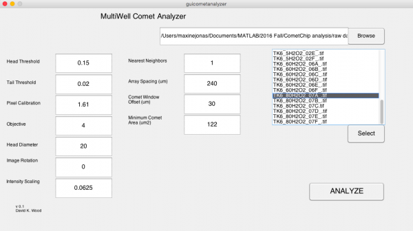     Multiwell Comet Analyzer window.
4. Click Browse.
   • Select the stacked image directory you created in the previous section.
   • Click Open.
     

     

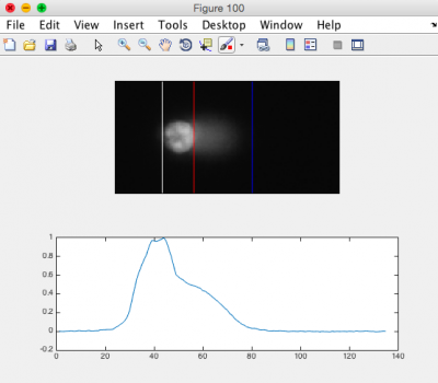     CometChip analysis showing differentiation between head and tail.
5. From the image stack files loaded to the MultiWell Comet Analyzer window, choose ONE image that is expected to show DNA damage. You are just using this image to optimize the analysis parameters.
   • The chosen file should be highlighted.
   • Click Select.
6. Click Analyze.
7. Click "Yes" when the dialog box appears and asks if you want to run the program in "debug mode."
   • Please do not hit any additional keys until this process is completed.
   • In the MATLAB command window you will see the number of comets to be analyzed. The same number of figures should be generated.
8. Review the generated images.
   • Ensure that the head of the comet is bracketed by a white line on the left, and a red line on the right. The tail should be bracketed by the red line and a blue line on the right. See the image to the right for an example.
   • You may need to adjust the "Tail Threshold" value so that the tail is identified appropriately and/or the "Head Threshold" value so that the head is identified appropriately.
   • Note: it is okay if some of the images do not appear correct according to the above criteria; however, the majority of your images should be correct.
9. In the Command Window type "close all."
10. If you need to adjust your parameters, repeat this process again until you find the optimal parameters for your analysis.
    • Find the guicometanalzyer window.
    • Adjust parameters as needed and repeat steps above by continuing to run in "debug mode."
    • Type "close all" when done, but leave Matlab open.

Measure head and tail lengths using MATLAB

1. Find the guicometanalyzer window
   • If it has disappeared, run the script again by typing "guicometanalyzer" in the command window.
2. In the MultiWell Comet Analyzer window, confirm the parameters as above.
   • Click Browse.
   • Select the stacked image directory you created with ImageJ.
   • Click Open.
3. Highlight all stack files in the MultiWell Comet Analyzer window.
   • Click Select.
4. Click Analyze.
5. Click "No" when the dialog box appears and asks if you want to run the program in "debug mode."
6. Confirm that there is a .txt file for each stack in your folder.
   • Be sure to keep MATLAB open.

Compile results and export to Excel

1. In the command window, type "comettoexcel" and press enter to run the script.
2. When prompted, select the directory containing all the txt files that were output by guicometanalyzer and click "Open."
3. The script will compile all your data, calculate the median values for each well, and export the data in an Excel file.
4. Next, a dialog box will prompt you to save the Excel file.
5. Please choose an appropriate directory and file name to save your data.
6. Click "Save" and ensure your data has saved correctly.

Post your final Excel spreadsheets on the M1 main Discussion page.

• There should be one spreadsheet for the buffer control CometChip, and one for the enzyme-treated CometChip.

Part 3: In-class paper discussion

We will finish today with a discussion concerning the following research article:

Ge, J., Wood, D. K., Weingeist, D. M., Prasongtanakij, S., Navasumrit, P., Ruchirawat, M., and Engelward, B. P. Standard fluorescent imaging of live cells is highly genotoxic. (2013) Cytometry. 83A:552-560.

Our paper discussion will be guided by all that you have learned about how to write a cohesive story that clearly reports the data and provides strong support for the conclusions made about the data. During the paper discussion, everyone is expected to participate - either by volunteering or by being called upon!

Introduction

Remember the key components of an introduction:

• What is the big picture?
• Is the importance of this research clear?
• Are you provided with the information you need to understand the research?
• Do the authors include a preview of the key results?

Results

Carefully examine the figures. First, read the captions and use the information to 'interpret' the data presented within the image. Second, read the text within the results section that describes the figure.

• Do you agree with the conclusion(s) reached by the authors?
• What controls were included and are they appropriate for the experiment performed?
• Are you convinced that the data are accurate and/or representative?

Discussion

Consider the following components of a discussion:

• Are the results summarized?
• Did the authors 'tie' the data together into a cohesive and well-interpreted story?
• Do the authors overreach when interpreting the data?
• Are the data linked back to the big picture from the introduction?

Reagents list

• permeabilization buffer: 0.2% Triton in Tris buffer saline (TBS, Invitrogen)
• blocking buffer: 1% bovine serum albumin (BSA) in TBS
• primary antibody to γH2AX, mouse (Millipore)
• goat anti-mouse secondary antibody (Invitrogen)

Navigation links

Next day: Visualize and analyze data for sub-nuclear foci assay

Previous day: Complete biochemical experiment and apply chemical treatments for sub-nuclear foci assay