Difference between revisions of "Assignment 1, Part 2: Optics bootcamp"

This is Part 2 of Assignment 1.

Lab orientation

Welcome to the '309 Lab! It's time to get your hands dirty — time to get a little mens in your manus. Step one: go to the lab. (If you are already in the lab, proceed to the next step. By the way, your hands shouldn't be dirty. That's just an expression. If your hands really are dirty, then wash them with soap and water. You are going to be handling sensitive optics!)

Before you get started, take a little time to learn your way around.

Thorlabs CP02 vs CP02T

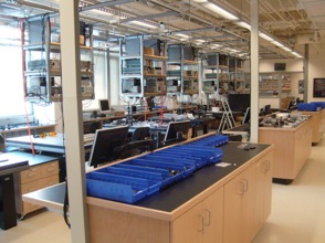
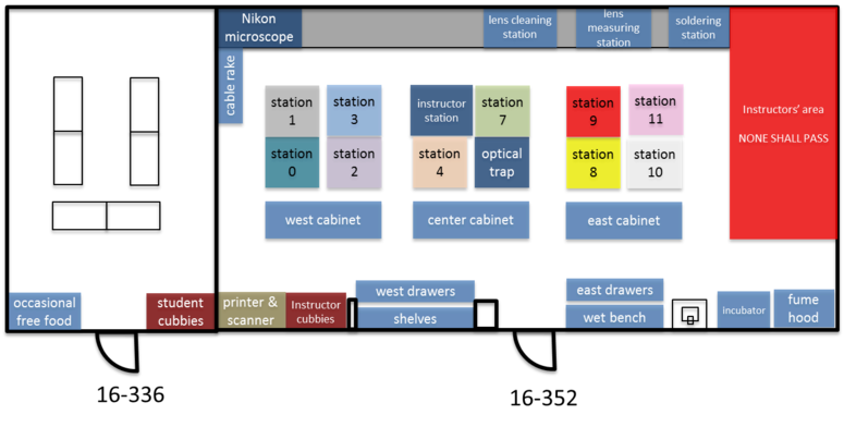
The 20.309 lab contains more than 15,000 optical, mechanical, and electronic components that you may choose from in order to complete your assignments throughout the semester. You can waste a lot of time looking for things, so take a little time to learn your way around. The floor plan below shows the layout of rooms 16-352 and 16-336. When you get to the lab, take a walk around, especially to the center cabinet, west cabinet, and west drawers. Go everywhere and check things out for a few minutes. Read the time machine poster near the printer. Discover the stunning Studley tool chest poster near the east parts cabinet.

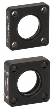
You probably noticed that many components are filed in boxes labeled with a sequence of letters and numbers. A company called Thorlabs manufactures the most of the optics and optical mounts you will use. The lab manuals frequently refer to components by their part number, which is usually one or two letters that have a vague relationship to the name of the part, followed by a couple of numbers. For example, the Thorlabs part number for a certain type of cage plate is "CP02." Thorlabs makes many kinds of cage plates, each with a subtle variation in its design. All of the cage plate part numbers starts with the letters "CP," followed by some numbers and in some cases a letter or two at the end. The Thorlabs website has an overview page of various kinds of cage plates here. Googling "Thorlabs CP02" is a quick way to get to the catalog page for that part.

To the untrained eye, many of the components in the lab are indistinguishable. The picture on the right shows just one example of strikingly-similar-looking bits. Take care when you select components from stock. Students sometimes return components to the wrong bins. Use even more care when you put things away. It is helpful to sing the One of These Things is Not Like the Others song from Sesame Street out loud while you are putting things away to ensure that you don't make any errors. (For the final exam, you will be required to identify various components while blindfolded.)

Note that Station 9 is now the "Instructor Station," and the previously labeled instructor station is now "Station 5" and available for your use.

See! Wasn't that a worthwhile journey?

Exercise 1: measure focal length of lenses

Make your way to the lens measuring station. Measure the focal length of the four lenses marked A, B, C, and D located nearby.

Report the focal length you measured for each lens A through D.

Exercise 2: imaging with a lens

Imaging apparatus with illuminator, object, lens, and CMOS camera mounted with cage rods and optical posts.

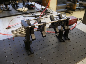
Make your way to the pre-assembled lens setup that looks like the thing on the right. You will be using similar parts to build your microscope, so take some time to look at the construction of the apparatus. Identify the illuminator, the object (a glass slide with a precision micro ruler pattern on it), the imaging lens (a, f=35mm, biconvex lens mounted in a lens tube), and the camera (where the image will be captured). All of the components are mounted in an optical cage made out of cage rods and cage plates. The cage plates are held up by optical posts inserted into post holders that are mounted on an optical breadboard that sits on top of a vibration reducing optical table. You can adjust the positions of the object and lens by sliding them along the cage rods.

In this part of the lab, you will use this simple imaging system with one lens to compare measurements of the object distance $ S_o $, image distance $ S_i $, and magnification $ M $ with the values predicted by the lens makers' formula:

$ {1 \over S_o} + {1 \over S_i} = {1 \over f} $

$ M = {h_i \over h_o} = {S_i \over S_o} $

Make a block diagram of the apparatus (a legible, hand drawn sketch is fine). You do not need to detail the mechanical construction, but be sure to include all of the optical elements: light source, lenses, camera, and object. Indicate $ S_i $ and $ S_o $ on the diagram.

Measure stuff

• If the LED is not already on, verify that the power supply current limit is set to a number less than 0.5 A, and press the OUTPUT button. You should see red light coming from the LED.
• Move the imaging lens as close to the camera as it will go. The illuminator lens should be about 10 to 15 mm away from the LED.
• Launch MATLAB.
• In the command window, start the image acquisition tool by running the following two lines of code:

foo = UsefulImageAcquisition;
foo.Initialize

Figure 1: Side view of the Manta G-040 CMOS camera. The detector is recessed inside the body of the camera, 17.5 mm from the end of the housing. The detector comprises an array of 728x544 square pixels, 6.9 μm on a side. The active area of the detector is 5.02 mm (H) × 3.75 mm with a diagonal measurement of 6.3 mm. The manual for the camera is available online here.

• After the Image Acquisition window appears, click the Start Preview button.
• Set the exposure time:
• Set Gain = 0, Frame Rate = 20, Black Level = 0, and Number of Frames = 1 for now.
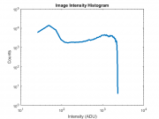
• Set Exposure to obtain a properly exposed image. When you have the setting right, there should be a wide range of pixel values — from dark to light — and no overexposed pixels. The histogram plot is useful for assessing the exposure. The horizontal axis shows all of the possible pixel values, from completely dark to the brightest white. The vertical axis indicates the number of pixels at each value. (The units of the exposure setting are in microseconds.)
  • You can also adjust the LED current to obtain a good exposure. DO NOT EXCEED 0.5 A.
• Move the object to produce a focused image.
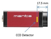
• Measure the distance $ S_o $ from the target object to the lens and the distance $ S_i $ from the lens to the camera detector.
  • Figure 1 shows the location of the detector inside of the camera.
• In the image acquisition window, press Acquire (lower right).
• Save your image to the MATLAB workspace
  • Every time you press Acquire, the image data appears in a property of foo called ImageData. Use a "dot" to access properties. Note that this property gets overwritten every time you press Acquire, so you have to save the data somewhere else if you want to work with it later on.
  • MATLAB has a top level context called the workspace where you can save variables and work with them from the command line. Choose a descriptive variable name such as ImageSo50mm and assign it to foo.ImageData using the equals symbol: ImageSo50mm = foo.ImageData. If you'd like to see a list of the variables in the workspace, type who on the command line.
• Compute the magnification.
  • One operation on images you will do frequently is to adjust their contrast. You can define a simple function that will save a bunch of typing each time you want to do this. MATLAB supports a thing called inline function declaration. Type: StretchContrast = @(ImageData) ( double( ImageData ) - min( double( ImageData(:) ) ) / range( double( ImageData(:) ) ). Don't sweat the details of this for now. We will talk about it in class, soon.
  • In the MATLAB Command Window, display your image by typing figure; imshow( StretchContrast( Image1 ) );
  • Go back to the command window (by pressing ALT-TAB on the keyboard or selecting it from the task bar) and type imdistline.
  • Use the line to measure a feature of known size on the micro ruler
    • The small tick marks are 10 μm apart
    • The large tick marks are 100 μm apart
    • The whole pattern is 1 mm long
    • The pixel size is 7.4 μm
• In a table, record $ S_o, S_i, h_o, h_i, $, and calculate the magnification M, for at least 4 image and object distances. Aim for an equal number with the target placed at less than and greater than 2$ f $ from the lens.
• Using MATLAB, or your other favorite plotting software, make a plot of $ {1 \over S_i} $ as a function of $ {1 \over f} - {1 \over S_o} $, and $ {h_i \over h_o} $ as a function of $ {S_i \over S_o} $

List up to three predominant sources of error that affected your measurements of $ S_o $ and $ S_i $ (i.e. What factors prevented you from making a more accurate or more precise measurement? The answer "human error" does not describe anything specific nor useful, and will not earn you any points.) Estimate the magnitude of each error that you listed. List one or two predominant sources of error that affected your measurements of $ h_i $. Estimate the magnitude of each error that you listed. Turn in your table of measured values for $ S_o, S_i, h_o, h_i, $ and $ M $. Turn in your plot of $ {1 \over S_i} $ as a function of $ {1 \over f} - {1 \over S_o} $. Turn in your plot of $ {h_i \over h_o} $ as a function of $ {S_i \over S_o} $. What did you expect each plot to look like based on the theory you learned in class? Did your plots meet your expectations? Why or why not?

Exercise 3: noise in images

Suppose you pointed a camera at a perfectly static scene where nothing at all was changing. The camera didn't move at all, the objects in the scene were perfectly stationary, and the lighting stayed exactly the same. To continue the thought experiment, say you made a really boring movie of this scene by taking, oh, 100 successive pictures of the scene at regular intervals. In an ideal world, you would expect that every frame of the movie would be exactly the same as all the others. Figure 2 depicts a dataset generated by this thought experiment as a mathematical function $ P_{x,y}[t] $. If there was no noise at all, the numerical value of each pixel in all 100 of the images would be the same in every frame:

$ P_{x,y}[t]=P_{x,y}[0] $,

where $ P_{x,y}[t] $ is the the pixel value reported by the camera of at pixel $ x,y $ in the frame that was captured at time $ t $. The square braces indicate that $ P_{x,y} $ is a discrete-time function. It is only defined at certain values of time $ t=n\tau $, where $ n $ is the frame number and $ \tau $ is the interval between frame captures. $ \tau $ is equal to the inverse of the frame rate, which is the frequency at which the images were captured.

You probably can guess that IRL, this doesn't happen. (Spoiler alert.) All 100 frames will not be perfectly identical. We will talk in class about why this is so. For now, let's just measure the phenomenon and see what we get. A good way to make the measurement is to just go ahead and set up a static scene, take 100 pictures of it, and then compute how much each pixel varied over the course of the movie. Any variation in a particular pixel's value over time must be caused by random noise of one kind or another. Simple enough. (An alternate way to do this experiment would be to simultaneously capture the same image in 100 identical, parallel universes. This would obviously reduce the time needed to acquire the data. You are welcome to use this alternative approach, if you like.)

Capturing an image involves measuring light intensity at numerous locations in space. The Manta G-040 CMOS cameras in the lab measure 396,032 unique locations during each exposure. Every one of those measurements is subject to noise. In this part of the lab, you will quantify the random noise in images made with the these cameras, which are the same ones that you will use in the microscopy lab.

Figure 2: Noise measurement experiment. The cameras in the lab produce images with 728 horizontal by 544 vertical picture elements, or pixels. For each picture, the camera measures the intensity of light falling on each pixel and returns an array of pixel values $ P_{x,y}[t] $. The pixel values are in units of analog-digital units (ADU).

Figure 3: Pixel variance versus mean mystery plot. Can you stand the suspense?

We need a quantitative measure of noise. Variance is a good, simple metric that specifies exactly how unsteady a quantity is, so why not give that a try? (In case it's been a while, variance is defined as $ \operatorname{Var}(P)=\langle(P-\bar{P})^2\rangle $.)

So here's the plan:

• Set up a static scene that has a range of light intensities from bright to dark and point your camera at it.
• Make a movie of 100 frames.
• Compute the variance of each pixel over time.
• Make a scatter plot of each pixel's variance on the vertical axis versus its mean value on the horizontal axis, as shown in Figure 3.

Plotting the data this way will reveal how the quantity of noise depends on intensity. With zero noise, the plot would be a horizontal line on the axis. But you know that's not going to happen. How do you think the plot will look? This boring movie is getting more suspenseful all the time! I hope it doesn't have a scary ending.

Set up the scene and adjust the exposure time

The first step is to configure the camera settings. Enter "15" in the "Gain" box and "16" in the "Dark Level" box. These two settings control how $ P_{x,y} $ relates to the number of photons the camera detects. In general, $ P=G O $, where $ G $ is the gain, and $ O $ is the offset. To make things confusing, the numbers you type into the boxes are not the same as the values in the equation. If you set up the camera this way, $ G=1 $ and $ O=64 $. Why not?

Now set up a scene that has a large range of light intensities. One easy way to do this using the same apparatus you used in the previous part is to slide the 35 mm lens as far as it will go toward the camera. You should see a bright spot in the middle of the camera. Screw an iris in to the other side of the X-lookin' thing where the imaging target is mounted. Start with the iris most of the way open. Futz with the exposure, iris, and lens position until you have roughly the same number of pixels for each intensity value. Use the histogram plot to assess your setip. This useful plot tells you the distribution of pixel intensities in an image. The x-axis tells you the brightness of the pixel, and the y-axis tells you how many pixels have of that brightness. Maximize the range and even out the number of pixels at each intensity.

If you ever want to plot your own histogram from a saved image, here is some example MATLAB code to do just that:

[ counts, bins ] = hist( double( squeeze( exposureTest(:) ) ), 100);
semilogy( bins, counts, 'LineWidth', 3 )
xlabel( 'Intensity (ADU)' )
ylabel( 'Counts' )
title( 'Image Intensity Histogram' )

For this part of the lab, you will change your experimental set up to obtain an image with an approximately uniform intensity histogram. Lucky for you, the UsefulImageAcquisition tool displays the intensity histogram of your image in the top right corner of the Image Acquisition window, so you don't need to generate one each time you change something in your setup.

Figure 4: Example intensity histogram with approximately uniform distribution of pixel values over the range 10-2000 ADU.

1. In the Image Acquisition window, click Start Preview.
2. Set the Exposure property to 100.
3. Adjust your experiment until your histogram is a roughly uniform distribution of pixel values. Figure 4 shows a reasonably nice histogram.
   • Try to get a broad range of pixel values between about 10 and 2000. Try not to have any pixels that are over-exposed (i.e. your max pixel value is 4095 and you see a red 'x' on the preview histogram)
   • You may need to adjust the exposure time and LED current (but remember not to exceed 0.5 A!).
   • Be creative! In this case, we don't care exactly what the image looks like, we're just trying to get a large range from bright to dark. You can try sliding all the components around, or disconnecting the camera, whatever gets you the largest and flattest distribution of pixels.

Acquire movie and plot results

Once you are set up correctly, make a movie and plot the results using the procedure below:

1. Capture a 100 frame movie.
   • Go to the Image Acquisition window and change the Number of Frames property from 1 to 100.
   • Press Acquire.
   • Switch to the MATLAB console window. (Press alt-tab until the console appears.)
   • Save the movie to a variable called noiseMovie by typing: noiseMovie = foo.ImageData;
2. Plot pixel variance versus mean.
   • Use the code below to make your plot.

pixelMean = mean( double( squeeze( noiseMovie) ), 3 );
pixelVariance = var( double( squeeze( noiseMovie) ), 0, 3 );
[counts, binValues, binIndexes ] = histcounts( pixelMean(:), 250 );
binnedVariances = accumarray( binIndexes(:), pixelVariance(:), [], @mean );
binnedMeans = accumarray( binIndexes(:), pixelMean(:), [], @mean );
figure
loglog( pixelMean(:), pixelVariance(:), 'x' );
hold on
loglog( binnedMeans, binnedVariances, 'LineWidth', 3 )
xlabel( 'Mean (ADU)' )
ylabel( 'Variance (ADU^2)')
title( 'Image Noise Versus Intensity' )

Save your plot as a .png (on the plot, click on File -> Save As ->)

Plot pixel variance vs. mean. Describe how noise varies as a function of light intensity. (Notice that the axes of this plot are in log scale. Click here if you'd like a refresher how to interpret log-log plots.) Did the plot look the way you expected?

When you're done, please slide the object and lenses back to where you found them at the start of the lab exercise. Make sure you have all the relevant plots and/or data saved, then clear the MATLAB workspace for the next group using the command clear all.

Navigation

• Overview
• Part 1: Pre-lab questions
• Part 2: Optics bootcamp
• Part 3: Build a microscope
• Part 4: Measure stuff

Back to 20.309 Main Page