20.109(F16):Seed cells for immuno-flourescence assay (Day5)

Introduction

H2AX assay information...

Protocols

Today you will begin the initial steps for the γH2AX assay and complete the final steps of your CometChip assay. The teaching faculty will tell you which exercise to complete first.

Part 1: Seed cells for H2AX assay

To prepare for the H2AX assay, you will first seed wells within two 12-well plates. The cells will incubate for 24 h, then one plate will be exposed to gamma-irradiation. The second plate will serve as the 'no treatment' control. When you return for the next laboratory session, you will compare the number of γH2AX foci in the gamma-irradiated samples to the number of foci in the control samples.

The steps below will be completed in the tissue culture room. Before you begin your work at the biosafety cabinet, the teaching faculty will lead you through a demonstration detailing how you will prepare your cells for seeding.

1. Obtain two 12-well plates from the teaching faculty.
   • Clearly label both plates - label one plate 'gamma-irradiated' and one 'control' in addition to your group information.
2. Add 0.5 mL of pre-warmed gelatin to each well of the top two rows (A1-A4 and B1-B4) of each plate.
3. Carefully place a coverslip into each well.
   • To ensure the coverslip settles at the bottom of the well, use a clean pipet tip to gently press down on the coverslip.
4. Move your 12-well plates to the 37 °C incubator.
5. You will seed each well with 100,000 cells according to the procedure demonstrated by the teaching faculty.
   • Obtain a flask of A549 cells from the 37°C incubator.
     • Observe the color and clarity of the media. Fresh media is reddish-orange in color and if the media on your cells is yellow or cloudy, it could mean that the cells are overgrown, contaminated, or starved for O₂.
     • Next look at the cells on the inverted microscope. Note their shape and arrangement in the dish and how densely the cells cover the surface.
   • Gather aliquots of 1x PBS, trypsin and fresh media from the 37°C waterbath.
     • One of the greatest sources for TC contamination is moving materials in and out of the hood since this disturbs the air flow that maintains the sterile environment inside the hood. Anticipate what you will need during your experiment to avoid moving your arms in and out of the hood while your cells are inside.
   • Aspirate the media from the flask.
   • Add 3 mL of 1x PBS to the flask and rock from side to side, then aspirate.
   • Add 0.7 mL of trypsin to the flask and rock from side to side to ensure the bottom is coated, then incubate the flask in the 37°C incubator for 2 min.
   • Retrieve your flask from the incubator and firmly tap the bottom of the flask 3-5 times.
     • Examine the cells using the microscope. Detached cells will be rounded and float in the liquid. If your cells are not detached from the flask, return the flask to the 37°C incubator for an additional 2 min.
   • Add 2 mL fresh media to the flask and pipet the liquid up and down (“triturate”) to suspend the cells.
6. Use a hemocytometer to determine the concentration of your cells.
   • Transfer 90 μL of the cell suspension to an eppendorf tube.
   • Add 10 μL of Trypan blue.
   • Pipet 10 μL of the cell/dye mix to the hemocytometer and count the cells as you did during the Orientation exercise.
   • Multiply the average number of cells within the four corner squares by 10,000 to determine the number of cells/mL.
7. Either dilute or concentrate your cell suspension such that 1 mL contains 100,000 cells.
   • If you are unsure how to proceed here, ask your teaching faculty for assistance.
8. Retrieve your 12-well plates from the incubator and aspirate the gelatin from the wells.
9. Add 1 mL of cell suspension to each well that was treated with gelatin.
   • Check that the coverslip does not float to the surface.
10. Return your 12-well plates to the 37°C incubator.

In ~24 h, Marcus Parrish from the Engelward Laboratory will expose your experimental plates to 60 Gy of gamma-irradiation for 1 min. The cells will then recover at 37°C for 30 min. During the recovery incubation the γH2AX foci will form at the sites of DNA double strand breaks. Following recovery, the teaching faculty will fix the cells by adding 4% formaldehyde for 10 min. This step stops the repair process without disrupting the foci that have formed. Lastly, the fixed cells will be washed with 1x PBS and stored at 4 °C until your next laboratory meeting.

Part 2: Data analysis for CometChip assay

Stack images using ImageJ

1. Open ImageJ from Applications.
2. Go to Plugins → Macros → Run...
3. Select script "GenImageStacks_singleimage.txt"
   • Find within the "Fa16 CometChip Analysis" subfolder in MATLAB.
4. Choose as a source directory enter file name .
   • Find within the "Fa16 CometChip Analysis" subfolder in MATLAB.
5. Create a destination directory titled enter file name _stacked by selecting New Folder.
6. Click Choose.
   • ImageJ will create the stacked images in ~2 min.
   • Please do not hit any additional keys until this process is completed.
7. Confirm that the stacks are in the destination directory.
   • Open enter file name _stacked.
   • You should see one .tif image stack per well.
8. Close ImageJ.

Optimize analysis parameters using MATLAB

1. Open MATLAB from Applications.
   • Be sure that "Fa16 CometChip Analysis" is the current folder.
2. Double click "guicometanalyzer.m" to open the script in the editor window.
3. Find 'debug' in the script.
4. Select the code from lines 645-652.
   • Use the keyboard short cut "Command + t" to uncomment.
5. At this point it is very important to save!
6. In the command window, type "guicometanalyzer".
   • Press return key.
7. In the MultiWell Comet Analyzer window:
   • Check that the Pixel Calibration value is 1.61.
   • Check that the Image Rotation value is 0.
   • Check that the Array Spacing (μm) is 240.
   • Check that the Head Diameter value is 20.
   • Confirm the settings with the image below.
     

     

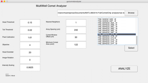     Multiwell Comet Analyzer window.
8. Click Browse.
   • Select enter file name _stacked.
   • Click Open.
     

     

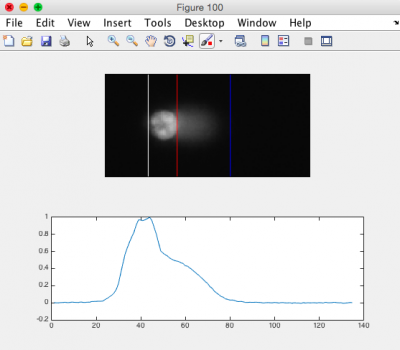     CometChip analysis showing differentiation between head and tail.
9. From the image stack files loaded to the MultiWell Comet Analyzer window, choose one that is expected to show DNA damage.
   • The chosen file should be highlighted.
   • Click Select.
10. Click Analyze.
    • Please do not hit any additional keys until this process is completed.
    • In the MATLAB Command Window you will see the number of comets to be analyzed. The same number of figures should be generated.
11. Review the generated images.
    • Ensure that the head of the comet is bracketed by a white line on the left, and a red line on the right. The tail should be bracketed by the red line and a blue line on the right. See the image to the right for an example.
    • Note: it is okay if some of the images do not appear correct according to the above criteria; however, the majority of your images should be correct.
12. In the Command Window type 'close all'.
    • Be sure to keep MATLAB open.

Measure head and tail lengths using MATLAB

1. Select the code from lines 645-652.
   • Use the keyboard short cut "Command + /" to comment out.
2. At this point it is very important to save!
3. In the command window, type "guicometanalyzer".
   • Press return key.
4. In the MultiWell Comet Analyzer window, confirm the parameters as above.
   • Click Browse.
   • Select enter file name _stacked.
   • Click Open.
5. Highlight all stack files in the MultiWell Comet Analyzer window.
   • Click Select.
6. Click Analyze.
7. Confirm that there is a .txt file for each stack in enter file name _stacked.
8. Exit MATLAB.

Compile results using Python

1. From the "Fa16 CometChip Analysis" subfolder in MATLAB, double click on "comettoexcel_gui.command" to launch Python program.
2. As your source directory, select enter file name _stacked.
   • Click Choose.
     

     

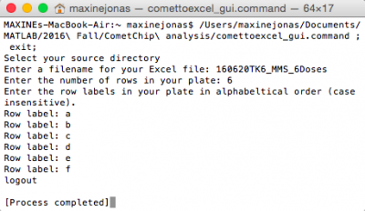     comettoexcel_gui.command window.
3. Enter information as follows:
   • Enter a filename for your excel file: " enter file name ".
     • Press return key.
   • Enter the number of rows in your plate: 6.
     • Press return key.
   • Enter the row labels in your plate in alphabetical order (case insensitive). Row label: a.
     • Press return key.
   • Row label: b.
   • Repeat to row label = f.
4. Press return key.
   • After a few seconds, "logout" will appear in Terminal Window.
5. In the enter file name _stacked folder, you should have an .xlsx summary file of your data.

Reagents

Navigation links

Next day: Complete immuno-fluorescence assay

Previous day: Assess repair variability with CometChip