Spring 2020 Assignment 9

Second-order systems

The Frequency Dependence of Osmo-Adaptation in Saccharomyces cerevisiae

Read [The Frequency Dependence of Osmo-Adaptation in Saccharomyces cerevisiae] and the [supporting information.]. This paper will be the focus of exam 2. We will discuss the paper and the supporting information on Thursday and Friday.

{{Template:Assignment Turn In|message = Answer the following questions about The Frequency Dependence of Osmo-Adaptation in S. cerevisiae:

1. What is the primary mechanism by which S. cerevisiae recovers from hyperosmotic shock?
2. What model did Mettetal, et. al. use for Hog1 activation in response to a hyperosmotic shock?
3. Mettetal, et. al. found that that the hyperosmotic shock response of wild-type yeast was (choose one): underdamped, critically damped, or overdamped.
4. The response of the mutant (low Pbs) yeast was (choose one): underdamped, critically damped, or overdamped.
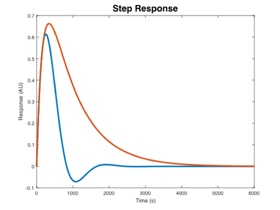
5. In the plot below, indicate which step response corresponds to the wild-type strain and the mutant strain.









Our goal for assignment 10 is to reproduce the bode plot in the paper (Figure 2 B and C), and fit it to a model second-order system. We will only measure the 'wild type' yeast strain, since measuring the mutant would take too much time. What mathematical model did Mettetal, et. al. use for the yeast response network? Express the model in the following forms: transfer function (TF), poles and zeros (ZPK), single differential equation (SDE), and coupled differential equations (CDE). Express the TF, SDE, and ZPK models in terms of the undamped natural frequency, $ \omega_0 $, damping ratio $ \zeta $, and/or damped natural frequency $ \omega_D $. Find an expression for the step response and plot it over a range of values of $ \omega_0 $ and $ \zeta $. A hand-drawn plot is fine, but you should probably look into MATLAB's step function. Plot the frequency response (i.e. make a Bode plot) of the system over a range of $ \omega_0 $ and $ \zeta $ values that includes over damped, critically damped, and under damped. What are two questions that you have about the paper's methodology or how we're going to implement the experiment in 20.309?




Yeast image analysis code

Download the data provided in the class dropbox folder. This data was collected by 20.309 students last semester. The movies were collected using the same 20.309 microscope that you built in class with an upgrade (that you would have done in Assignment 8 had we been on campus...) to incorporate a second fluorescence color. During an experiment, the microscope first recorded an image with blue illumination (exciting GFP) followed by one with green illumination (exciting RFP). It had a 40x objective and a 125 mm tube lens - remember that results in a 25x magnification.

The sample is similar to the one in Mettetal et al.: we are using S. cerevisiae with the protein Hog1 fused to GFP (which is excited by blue light) and an mRNA binding protein (we'll call MCP) fused to tagRFP (which is excited by green light) to locate the nucleus. A solenoid valve controls whether or not the medium provided to the yeast cells contains a high salt concentration, and in the experiment we oscillate between a high and low salt medium at a fixed rate. We expect to see the yeast cells 'respond' to an osmotic shock as a more localized Hog1-GFP signal that overlaps with the signal from the nucleus (RFP). Our goal is to calculate the average correlation coefficient between Hog1 and the nucleus as a function of the high/low valve state.

Load some data into MATLAB:

load('fall2019_StudentData_1');

The data is stored in a struct called yeastOsmoticShockData.

  
yeastOsmoticShockData = 

  struct with fields:

                         Movie: [544×728×2×16 uint16]
                          Time: [16×2 double]
                    ValveState: [16×2 logical]
        ValveOscillationPeriod: 960
     BlueCameraGainAndExposure: [6 5000000]
    GreenCameraGainAndExposure: [15 5000000]

The data structure contains all the important information from the experiment:

• yeastOsmoticShockData.Movie is a two-color movie, where the 3d dimension is the color (1 = Blue excitation = GFP, 2 = Green excitation = RFP), and the fourth is the frame number. Notice that yeastOsmoticShockData.Movie is a uint16 data type which is the same as the movies you worked with in the particle tracking assignments.
• yeastOsmoticShockData.Time is the time stamp of each frame, recorded in seconds from the start of the experiment. Column 1 contains the timestamps of the GFP images, column 2 is for the RFP images.
• yeastOsmoticShockData.ValveOscillationPeriod is the oscillation valve period, in seconds.
• yeastOsmoticShockData.BlueCameraGainAndExposure and yeastOsmoticShockData.GreenCameraGainAndExposure are the blue and green illumination camera settings in the format [gain, exposure], where exposure is in microseconds.
• yeastOsmoticShockData.ValveState is the state of the solenoid pinch valve controlling the salt concentration at the time of each image. The valve state is 0 for low salt, and 1 for high salt. If you need to know the valve state more precisely, it can be calculated with the following conditional statement: $ sin(2 \pi t/T) \ge 0 $, where T is the valve oscillation period, and t is the time since the start of the experiment (this is how the state is determined in the software).




Choose a single frame of the movie. Make a four panel figure and display: the GFP image, the RFP image (both with a scale bar), and their corresponding image histograms. Include an appropriate title for each panel.




Analyze a frame

In each frame of our movie, we need to locate and identify individual cells, and find the correlation coefficient between the cell image and the nuclei image. If the Hog1 signal is localized in the nucleus, the correlation should be close to 1, while if there is no correlation between the signals, the correlation will be close to zero. In reality, we'll likely see correlations close to about 0.5, but we'll look for an increase or decrease in the signal to determine the amount of Hog1 localization.




Start with the following basic layout of the function:

function [AverageNucleusHog1Correlation, StandardErrorNucleusHog1Correlation] = AnalyzeFrame( TwoColorFrame, BackgroundImage, BackgroundRectangle )

     % 1. estimate the background level
backgroundScaleFactors = FindBackgroundScaleFactor(TwoColorFrame,BackgroundImage, BackgroundRectangle);

cellFrame = TwoColorFrame(:,:,1) - backgroundScaleFactors(1)*BackgroundImage(:,:,1);
nucleiFrame = TwoColorFrame(:,:,2) - backgroundScaleFactors(2)*BackgroundImage(:,:,2);

     % 2. identify individual yeast cells in the GFP image
     % 3. calculate the correlation coefficient between the GFP intensities an RFP intensities within each cell region
     % 4. output the mean correlation coefficient for all cells in the frame

end

As you work through this part of the Assignment, fill out the AnalyzeFrame function to incorporate each of the outlined steps.

Finding cells

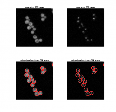
We could consider using a threshold to identify cells in an image, similar to how we found fluorescent particles in Assignments 4 and 5. The problem here, is that thresholding doesn't allow us separate a single cells from a clump of cells. Since we know that yeast cells are roughly spherical, we can use imfindcircles to locate them. imfindcircles is an implemenattion of the Hough transform.

     [cellCenters, cellRadii] = imfindcircles(cellFrame,[Rmin Rmax],'ObjectPolarity','bright','Sensitivity',0.95);

Here, Rmin and Rmax are the smallest and largest expected 'radii'. How can you estimate Rmin and Rmax?

The function viscircles(cellCenters,cellRadii) may be useful to visualize your results.

Loop through each cell and calculate the correlation coefficient between GFP and RFP

Next we want to calculate the response of the Hog1 protein. In the paper, they calculated the response as the ratio of GFP intensities inside and outside the nucleus: $ R_{Hog1} = \frac{<GFP_{nucleus}>}{<GFP_{cell}>} $. We'll use an alternative way to find the response: by finding the correlation coefficient between the GFP and RFP signals within each cell.

Finish filling out AnalyzeFrame to loop through each circle found in the frame and extract the corresponding pixel intensities from your GFP and RFP images. Then, calculate the correlation coefficients between these two intensity vectors (corr in MATLAB). The following helper function may be useful.

function Im = createMaskFromCircles(centers,radii,ImageSize)
    Im = zeros(ImageSize);
    [X, Y] = meshgrid(1:ImageSize(2), 1:1:ImageSize(1));

    for ii = 1:length(radii)
        isBright = (X-centers(ii,1)).^2+(Y-centers(ii,2)).^2 <= radii(ii,1)^2;
        isAlreadyFound = (Im == 1);
        Im = Im + (isBright & ~isAlreadyFound);
    end
    Im( Im > 1 ) = 1;
end

Once you've collected each individual correlation coefficient, find the mean and standard error, and output these from the function.

Analyze the movie

Once you've set up your analysis for a single frame, you'll now want to loop through the movie and collect the responses as a function of time.




Analyze each frame of the movie and plot the average cellular response as a function of time. In a single figure, plot the data in one subplot, and the pinch valve state (1 for high salt, 0 for low salt) in a second subplot. Write a function to fit the response to a sinusoid and extract the predicted amplitude and phase shift of the response signal. Plot the best fit function on the same plot as your data. Report the resulting best fit parameters.








Turn in all your MATLAB code in pdf format. No need to include functions that you used but did not modify.




Navigation

• Overview
• Part 1: Analyze a two-color yeast movie frame

Back to 20.309 Main Page

</div>