Difference between revisions of "Spring 2020 Assignment 9"
(→Yeast experiment data) |
MAXINE JONAS (Talk | contribs) (→Yeast experiment data) |
||
| Line 140: | Line 140: | ||
==Yeast experiment data== | ==Yeast experiment data== | ||
| − | Unfortunately, we won't be collecting our own data in the lab this semester, but it's still important to get a feel for what the raw data | + | Unfortunately, we won't be collecting our own data in the lab this semester, but it's still important to get a feel for what the raw data look like and how the signal manifests itself in those images. |
* Download the data file <tt>'fall2019_StudentData_3.mat'</tt> from the [https://www.dropbox.com/sh/j9gdbaoypukdydd/AACP1c3w6JzyzAa--XVpgMV0a?dl=0 Assignment 9 folder] in the course dropbox. The file contains raw data collected by 20.309 students during the Fall 2019 semester. | * Download the data file <tt>'fall2019_StudentData_3.mat'</tt> from the [https://www.dropbox.com/sh/j9gdbaoypukdydd/AACP1c3w6JzyzAa--XVpgMV0a?dl=0 Assignment 9 folder] in the course dropbox. The file contains raw data collected by 20.309 students during the Fall 2019 semester. | ||
| Line 173: | Line 173: | ||
A way to visualize the Hog1 and the nuclear protein simultaneously is to combine the two images into a single color color movie. The code below shows the GFP in cyan and the RFP in red. Areas of high overlap appear white. The code normalizes each frame to optimize the display contrast. It also overlays a square indicator in the upper left corner of the image — green for low salt and red for high salt. | A way to visualize the Hog1 and the nuclear protein simultaneously is to combine the two images into a single color color movie. The code below shows the GFP in cyan and the RFP in red. Areas of high overlap appear white. The code normalizes each frame to optimize the display contrast. It also overlays a square indicator in the upper left corner of the image — green for low salt and red for high salt. | ||
| + | |||
| + | * ''Tip!'' You can replay the movie in slow motion by changing the replay frame rate! In the movie player window, simply go to the Playback tab, click on Frame Rate... and change the playback frame rate (from 20 fps = 'real time' like the original source movie) to 1 frame per second for instance. | ||
<pre> | <pre> | ||
Revision as of 23:11, 28 April 2020
Signals and systems
| System function | $ \frac{1}{s+1} $ | $ \frac{s}{s+1} $ | $ \frac{s}{s^2+2s+1} $ | $ \frac{s}{s^2+0.1s+1} $ | $ \frac{1}{s^2+10s+1} $ |
|---|---|---|---|---|---|
| Magnitude plot | |||||
| Phase plot | |||||
| Step response | |||||
| Pole/zero plot | |||||
| Description |
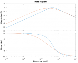
Magnitude Plots
Phase Plots
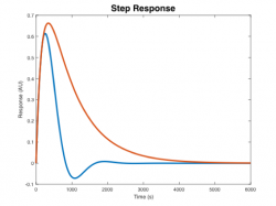
Step Response Plots
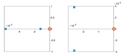
Pole Zero Plots
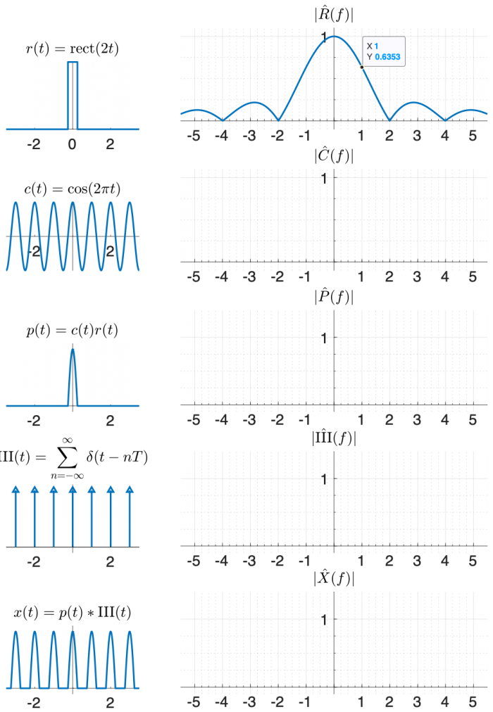
 One way to create x(t) using functions that appear on the transform table is:
- multiply a cosine by a rectangle, and then
- convolve the result with the comb function $ \mathrm{III(}t)=\sum\limits_{n=-∞}^{∞} \delta(t-nT) $.
Use the diagram below to help you find the answer. The left column of shows signals in the time domain, and the right column shows the magnitude of the Fourier transform of each signal. The top right plot is filled in for you, plus a little hint that might help you make an accurate plot.
(The phase of the transforms in this problem is zero at all frequencies, so it is not plotted.)
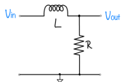
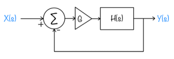
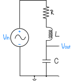
Feedback systems
|
|
The Frequency Dependence of Osmo-Adaptation in Saccharomyces cerevisiae
| |
Read The Frequency Dependence of Osmo-Adaptation in Saccharomyces cerevisiae and the supporting information.. This paper will be the focus of exam 2. We will discuss the paper and the supporting information on Thursday and Friday (4/30 and 5/1). Answer the following questions about The Frequency Dependence of Osmo-Adaptation in S. cerevisiae:
</div> |
|
|
|
Yeast experiment data
Unfortunately, we won't be collecting our own data in the lab this semester, but it's still important to get a feel for what the raw data look like and how the signal manifests itself in those images.
- Download the data file 'fall2019_StudentData_3.mat' from the Assignment 9 folder in the course dropbox. The file contains raw data collected by 20.309 students during the Fall 2019 semester.
- Load the file into your MATLAB workspace. You should see a variable called yeastOsmoticShockData, a struct which contains the movie data plus other relevant experimental parameters:
>> yeastOsmoticShockData

yeastOsmoticShockData =

  struct with fields:

                         Movie: [544×728×2×32 uint16]
                          Time: [32×2 double]
                    ValveState: [32×1 logical]
        ValveOscillationPeriod: 480
     BlueCameraGainAndExposure: [3 5000000]
    GreenCameraGainAndExposure: [15 5000000]
The engineered cells we used had 2 fluorescent proteins: a Hog1-GFP fusion and a nuclear protein tagged with RFP. Accordingly, the movie data has 2 color planes. The size of the movie's third dimension is 2. (It was 1 for the monochrome images we took in lab earlier this semester.)
- Color plane 1 is the GFP-Hog1 image, taken with blue illumination and green emission.
- The second color plane shows the RFP nuclear tag protein, taken with yellow/green illumination and red emission filters.
Use implay to watch each color of the movie:
implay(double(yeastOsmoticShockData.Movie(:,:,1,:))/4095);
implay(double(yeastOsmoticShockData.Movie(:,:,2,:))/4095);
Can you see how the distribution of Hog1 changes when the cell undergoes osmotic shock?
A way to visualize the Hog1 and the nuclear protein simultaneously is to combine the two images into a single color color movie. The code below shows the GFP in cyan and the RFP in red. Areas of high overlap appear white. The code normalizes each frame to optimize the display contrast. It also overlays a square indicator in the upper left corner of the image — green for low salt and red for high salt.
- Tip! You can replay the movie in slow motion by changing the replay frame rate! In the movie player window, simply go to the Playback tab, click on Frame Rate... and change the playback frame rate (from 20 fps = 'real time' like the original source movie) to 1 frame per second for instance.
close all

combinedMovie = zeros( size( yeastOsmoticShockData.Movie ) + [ 0 0 1 0 ] );
normalize = @( x ) ( x - min( x(:) ) ) / range( x(:) );

for ii = 1: size( yeastOsmoticShockData.Movie, 4 )
  gfpImage = normalize( double( yeastOsmoticShockData.Movie(:,:,1,ii) ) );
  gfpImageWithIndicator = gfpImage;
  gfpImageWithIndicator(10:50,10:50) = 1 - yeastOsmoticShockData.ValveState(ii);
  rfpImage = normalize( double( yeastOsmoticShockData.Movie(:,:,2,ii) ) );
  rfpImageWithIndicator = rfpImage;
  rfpImageWithIndicator(10:50,10:50) = yeastOsmoticShockData.ValveState(ii);
  combinedMovie(:,:,:,ii) = cat( 3, rfpImageWithIndicator, gfpImageWithIndicator, gfpImage );
end

implay( combinedMovie )


