Difference between revisions of "Optics Bootcamp"
Maxine Jonas (Talk | contribs) m (→Visualize, capture, and save images in Matlab) |
Juliesutton (Talk | contribs) (→Acquire movie and plot results) |
||
| (243 intermediate revisions by 6 users not shown) | |||
| Line 3: | Line 3: | ||
[[Category:Optical Microscopy Lab]] | [[Category:Optical Microscopy Lab]] | ||
{{Template:20.309}} | {{Template:20.309}} | ||
| + | [[File:Mens et Manus.jpg|center|350 px]] | ||
| + | <center> | ||
| + | <blockquote> | ||
| + | <div> | ||
| + | ''[https://www.youtube.com/watch?v=O7oD_oX-Gio You got your ''mens'' in my ''manus.]'' | ||
| + | <blockquote> | ||
| + | ''—[http://latin-dictionary.net/search/latin/mens Manus]'' | ||
| + | </blockquote> | ||
| + | </div> | ||
| + | </blockquote> | ||
| − | [ | + | <blockquote> |
| − | + | <div> | |
| + | ''[https://www.youtube.com/watch?v=GuENAWds5B0 You got your ''manus'' in my ''mens.]'' | ||
| + | <blockquote> | ||
| + | ''—[http://latin-dictionary.net/search/latin/manus Mens]'' | ||
| + | </blockquote> | ||
| + | </div> | ||
| + | </blockquote> | ||
| + | </center> | ||
==Overview== | ==Overview== | ||
| − | + | You are going to build a microscope next week. The goal of the Optics Bootcamp exercise is to make that seem like a less intimidating task. The bootcamp mixes a little bit of ''mens'' and a little bit ''manus''. It starts with a few written problems, followed by some exercises in the lab. The written problems will help you with the lab work. After you do the problems, come on by the lab. (Or do the problems in lab if you would like some help.) You will build an imaging apparatus made from some of the same optical components you will use in the microscopy lab, including an LED illuminator, an object with precisely spaced markings, a lens, and a CCD camera. You will compare measurements of object distance, image distance, and magnification to the values predicted by the lens makers' formula that was covered in class. You will also measure the noise characteristics of the CCD cameras we use in the lab. | |
| − | + | For a good review of geometrical optics, ray tracing, and some worked-out ray tracing examples, see [[Geometrical optics and ray tracing|this page]]. | |
| − | + | ||
| − | + | ==Problems== | |
| + | ===Problem 1: Snell's law=== | ||
| + | A laser beam shines on to a rectangular piece of glass of thickness <math>T</math> at an angle <math>\theta</math> of 45° from the surface normal, as shown in the diagram below. The index of refraction of the glass, ng, is 1.41 ≈√2. The index of refraction for air is 1.00. | ||
| − | [[ | + | [[File:Optics bootcamp snells law problem.png|center|300px]] |
| − | |||
| − | + | (a) At what angle does the beam emerge from the back of the glass? | |
| − | + | (b) When the beam emerges, in what direction (up or down) is it displaced? | |
| − | + | ||
| − | + | Optional: | |
| − | + | (c) By how much will the beam be displaced from its original axis of propagation? | |
| − | + | ||
| − | + | ===Problem 2: chelonian size estimation=== | |
| − | + | In the diagram below, an observer at height <math>S</math> above the surface of the water looks straight down at a turtle swimming in a pool. The turtle has length <math>L</math>, height <math>H</math>, and swims at depth <math>D</math>. <br> | |
| − | + | ||
| − | + | ||
| − | + | ||
| − | + | ||
| − | + | ||
| − | + | ||
| − | + | [[File:Turtle problem.png|center|350 px]] | |
| − | + | (a) Use ray tracing and Snell's law to locate the image of the turtle. Show your work. <br> | |
| − | + | (b) Is the image ''real'' or ''virtual''? <br> | |
| + | (c) Is the image of the turtle ''deeper'', ''shallower'', or ''the same depth'' as its true depth, <math>D</math>? <br> | ||
| + | (d) Is the image of the turtle ''longer'', ''shorter'', or ''the same length'' as its true length, <math>L</math>? <br> | ||
| + | (e) Is the image of the turtle ''taller'', ''squatter'', or ''the same height'' as its true height, <math>H</math>? | ||
| − | === | + | ===Problem 3: ray tracing with thin, ideal lenses=== |
| − | + | Lenses L1 and L2 have focal lengths of f1 = 1 cm and f2 = 2 cm. The distance between the two lenses is 7 cm. Assume that the lenses are thin. The diagram is drawn to scale. (The gridlines are spaced at 0.5 cm.) Note: Feel free to print out this diagram so you can trace the rays directly onto it. Or maybe use one of those fancy tablet thingies that the kids seem to like so much these days. | |
| + | <br /> | ||
| + | <br /> | ||
| + | [[File:RayTracing1.png|center|500 px]] | ||
| + | <br /> | ||
| − | + | (a) Use ray tracing to determine the location of the image. Indicate the location on the diagram. <br /> | |
| − | + | (b) Is the image upright or inverted? Is the image real or virtual? <br /> | |
| − | + | (c) What is the magnification of this system? <br /> | |
| − | + | ||
| − | + | ||
| − | + | Optional: | |
| − | + | ||
| − | + | (d) Lens L1 is made of BK7 glass with a refractive index n1 of 1.5. Lens L2 is made of fluorite glass with a refractive index n2 of 1.4. Compute the focal lengths of L1 and L2 if they are submerged in microscope oil (refractive index no = 1.5). | |
| − | + | ||
| − | === | + | ===Problem 4: this will be really useful later=== |
| − | + | In the two-lens system shown in the figure below, the rectangle on the left represents an unspecified lens L1 of focal length <math>f_1</math> separated by 0.5 cm from another lens L2 with focal length <math>f_2</math> of 1 cm. | |
| + | [[File:UnknownLens.png|center|500 px]] | ||
| − | + | Find the value of <math>f_1</math> such that all the rays incident parallel on this system will be focused at the observation plane, located at a distance d of 2 cm away from L2. | |
| − | == | + | ==Lab orientation== |
| − | + | Welcome to the '309 Lab. Before you get started, take a little time to learn your way around. | |
| + | {{:Lab orientation}} | ||
| − | + | ==Lab exercises== | |
| + | ===Lab exercise 1: measure focal length of lenses=== | ||
| + | Measure the focal length of the four lenses marked A, B, C, and D located near the lens measuring station. | ||
| − | = | + | <figure id="fig:Object_and_image_distance"> |
| − | + | [[Image: 20.309 130909 ImagingWithLens.png|thumb|right|300 px|<caption>Variables in the thin lens equation: object distance <math>S_o</math>, object height <math>H_o</math>, image distance <math>S_i</math>, and image height <math>H_i</math>.</caption>]] | |
| + | </figure> | ||
| − | + | ===Lab exercise 2: imaging with a lens=== | |
| + | In this part of the lab, you are going to build a simple imaging system with one lens and compare measurements of the object distance <math>S_o</math>, image distance <math>S_i</math>, and magnification <math>M</math> with the values predicted by the lens makers' formula: | ||
| − | + | :<math> {1 \over S_o} + {1 \over S_i} = {1 \over f}</math> | |
| − | + | ||
| − | + | ||
| − | + | ||
| − | + | :<math>M = {h_i \over h_o} = {S_i \over S_o}</math> | |
| − | + | <figure id="fig:Optics_bootcamp_apparatus"> | |
| + | [[Image: OpticsBootcampApparatus.png|thumb|right|300 px|<caption>Imaging apparatus with illuminator, object, lens, and CCD camera mounted with cage rods and optical posts.</caption>]] | ||
| + | </figure> | ||
| + | <xr id="fig:Optics_bootcamp_apparatus"/> is a picture of the thing you are about to build. From left to right, the apparatus includes an illuminator, an object (a glass slide with a precision microruler pattern on it), an imaging lens, and a camera to capture images. All of the components are mounted in an ''optical cage'' made out of ''cage rods'' and ''cage plates''. The cage plates are held up by ''optical posts'' inserted into ''post holders'' that are mounted on an ''optical table''. You will be able to adjust the positions of the object and lens by sliding them along the cage rods. | ||
| − | === | + | ====Gather materials==== |
| − | + | You can spend a huge amount of time walking around the lab just getting things in the lab, so it makes sense to grab as many parts as possible in one trip. <xr id="fig:Optics_bootcamp_apparatus"/> should give you some idea of what the parts look like. | |
| − | + | ||
| − | + | ||
| − | + | The materials you will need for this lab are shown in the image gallery below, including a part number and descriptive name of each component. When you come across a part name or number that is not-all-that-self-explanatory, remember that google is your friend. Most of the parts are manufactured by a company called ThorLabs. If you ever have a question about any of the components, the [http://www.thorlabs.com ThorLabs website] can be very helpful. For example, if the procedure calls for an SPW602 spanner wrench and you have no idea what such a thing might look like, try googling the term: "thorlabs SPW602". You will find your virtual self just a click or two away from [http://www.thorlabs.com/thorproduct.cfm?partnumber=SPW602 a handsome photo and detailed specifications]. | |
| − | + | <figure id="fig:Screw_gauge"> | |
| − | + | [[Image:Screw gauge.png|thumb|right|300 px|<caption>Screw measuring gauge and example screw specifications.</caption>]] | |
| − | | | + | </figure> |
| − | + | Screw sizes are specified as <''diameter''>-<''thread pitch''> x <''length''> <type>. The diameter specification is confusing. Diameters ¼" and larger are measured in fractional inches, whereas diameters smaller than ¼" are expressed as an [https://en.wikipedia.org/wiki/Unified_Thread_Standard#Designation integer number that is defined in the Unified Thread Standard]. The thread pitch is measured in threads per inch, and the length of the screw is also measured in fractional inch units. So an example screw specification is: ¼-20 x 3/4. [https://www.youtube.com/watch?v=lOoTpbxZQTY Watch this video] to see how to use a screw gauge to measure screws. (There is a white, plastic screw gauge located near the screw bins.) The type tells you what kind of head the screw has on it. We mostly use stainless steel socket head cap screws (SHCS) and set screws. If you are unfamiliar with screw types, take a look at the main screw page on the [http://www.mcmaster.com/#screws/=tjwmu5 McMaster-Carr website]. Notice the useful ''about ...'' links on the left side of the page. Click these links for more information about screw sizes and attributes. [http://www.boltdepot.com/fastener-information/printable-tools/Socket-Cap-Size-Chart.pdf This link] will take you to an awesome chart of SHCS sizes. | |
| − | + | ||
| − | + | ||
| − | + | ||
| − | + | ||
| − | + | ||
| − | + | ||
| − | + | ||
| − | + | ||
| − | + | ||
| − | + | ||
| − | + | ||
| − | + | ||
| − | + | ||
| − | + | ||
| − | + | ||
| − | + | ||
| − | + | ||
| − | + | ||
| − | + | ||
| − | + | ||
| − | + | ||
| − | + | ||
| − | + | ||
| − | + | ||
| − | + | ||
| − | + | ||
| − | + | ||
| − | + | ||
| − | + | ||
| − | + | ||
| − | + | ||
| − | + | ||
| − | + | ||
| − | + | ||
| − | + | ||
| − | + | ||
| − | + | ||
| − | + | ||
| − | + | ||
| − | + | ||
| − | + | ||
| − | + | ||
| − | + | ||
| − | + | ||
| − | + | ||
| − | + | ||
| − | + | ||
| − | + | ||
| − | + | ||
| − | + | ||
| − | + | ||
| − | + | ||
| − | + | ||
| − | + | ||
| − | + | ||
| − | + | ||
| − | + | ||
| − | == | + | =====Parts you will need for this lab:===== |
| + | <gallery widths=216px caption="Optical breadboard(Located in the lower left cubby of the Instructor Cubbies):"> | ||
| + | File:OpticalBreadBoard.jpg|Optical breadboard | ||
| + | </gallery> | ||
| − | + | <gallery widths=216px caption="Optomechanics (located in plastic bins on top of the center parts cabinet):"> | |
| + | File:LensTube05.jpg|2 x 0.5" Lens tube (SM1L05) | ||
| + | File:LCP01.jpg|2 x 2" Cage plate (LCP01, looks like an "O" in a square) | ||
| + | File:LCP02.jpg|4 x Cage plate adapter (LCP02, looks like an "X") | ||
| + | File:SM2RR.jpg|2 x 2" Retaining rings (SM2RR) | ||
| + | </gallery> | ||
| − | + | <gallery widths=216px caption="Optomechanics (located on the counter above the west drawers):"> | |
| − | + | File:ER8.jpg|3 x ER8 cage assembly rod (The last digit of the part number is the length in inches.) | |
| − | : | + | File:SM1RR.jpg|3 x 1" Retaining rings (SM1RR) |
| − | + | </gallery> | |
| − | + | ||
| − | + | <gallery widths=216px caption="Optics (located in the west drawers):"> | |
| − | + | File:Lenses.jpg|1 x LA1951 plano-convex, f = 25 mm lens (this will be used as a condenser for your illuminator) <br /> 1 x LB1811 biconvex, f = 35 mm lens (this will be used to form an image of your object) | |
| − | + | </gallery> | |
| − | + | ||
| − | + | ||
| − | + | ||
| − | + | ||
| − | + | ||
| − | + | ||
| − | + | ||
| − | + | ||
| − | + | ||
| − | + | ||
| − | + | ||
| − | + | ||
| − | + | ||
| − | + | ||
| − | + | ||
| − | + | ||
| − | = | + | <gallery widths=216px caption="Screws and Posts (located on top of the west parts cabinet):"> |
| − | + | File:PH2.jpg|3 x Post holders (PH2) | |
| − | + | File:TR2.jpg|3 x Optical posts (TR2) | |
| − | | | + | File:BA1.jpg|3 x Mounting base (BA1) |
| − | + | File:assortedScrews.jpg|3 x 8-32 set screws, <br />3 x ¼-20 x 1/4" or socket head cap screws, <br />4 x ¼-20 x 3/4;" socket head cap screws, <br />1 x ¼-20 set screw, <br />4 washers | |
| − | + | </gallery> | |
| − | + | ||
| − | + | ||
| − | + | ||
| − | + | ||
| − | + | ||
| − | + | ||
| − | + | ||
| − | + | ||
| − | + | ||
| − | + | ||
| − | + | ||
| − | + | ||
| − | + | ||
| − | + | ||
| − | + | ||
| − | + | ||
| − | + | ||
| − | + | ||
| − | + | ||
| − | == | + | <gallery widths=216px caption="More Parts (Located on top of the east cabinet):"> |
| − | * | + | File:NDfilter.jpg|1 x ND filter |
| − | * Plot <math>{1 \over S_i}</math> as a function of <math> | + | File:RedLED.jpg|1 x red, super-bright LED (mounted in heatsink) |
| − | * Plot <math>{h_i \over h_o}</math> as a function of <math>{S_i \over S_o}</math>. | + | File:MicroRuler.jpg|Microruler calibration slide mounted to a cage plate adapter |
| + | </gallery> | ||
| + | |||
| + | Most of the tools you will need are located in the drawers next to your lab station. Hex keys (also called Allen wrenches) are used to operate SHCSs. Some hex keys have a flat end and others have a ball on the end, called balldrivers. The ball makes it possible to use the driver at an angle to the screw axis, which is very useful in tight spaces. You can get things tighter (and tight things looser) with a flat driver. Here is a list of the tools you will need: | ||
| + | |||
| + | <gallery widths=216px caption="Tools (located in your station's drawers):"> | ||
| + | File:BallDrivers.jpg|1 x 3/16 hex balldriver for 1/4-20 cap screws <br/>1 x 9/64 hex balldriver, <br/>1 x 0.050" hex balldriver for 4-40 set screws (tiny) | ||
| + | File:SPW602.jpg|1 x SPW602 spanner wrench | ||
| + | </gallery> | ||
| + | |||
| + | You will also need to use an adjustable spanner wrench. The adjustable spanner resides at the lens cleaning station. There are only one or two of these in the lab. It is likely that one of your classmates neglected to return it to the proper place. This situation can frequently be remedied by yelling, "who has the adjustable spanner wrench?" at the top of your lungs. Try not to use any expletives. And please return the adjustable spanner wrench to the lens cleaning station when you are done. | ||
| + | |||
| + | <gallery widths=216px> | ||
| + | File:SPW801.jpg|1 x SPW801 adjustable spanner wrench | ||
| + | </gallery> | ||
| + | |||
| + | <gallery widths=216px caption="Things that should already be (and stay at) your lab station:"> | ||
| + | File:CCD.jpg|1 x Manta CCD cameraballdriver for 4-40 set screws (tiny) | ||
| + | File:cameraCables.jpg|1 x Calrad 45-601 power adapter for CCD, <br/>1 x ethernet cable connected to the lab station computer | ||
| + | </gallery> | ||
| + | |||
| + | ====Build the apparatus==== | ||
| + | Use the image of the apparatus to think about how to put your system together. The following guidelines should help get you started. If at any point you have questions, do not hesitate to ask an instructor for help. | ||
| + | |||
| + | =====Mount the LED===== | ||
| + | <center> | ||
| + | [[Image: 140729_OpticsBootcamp_05.jpg|frameless|x200px]] | ||
| + | [[Image: 140729_OpticsBootcamp_07.jpg|frameless|x200px]] | ||
| + | [[Image: AttachBA1.JPG|frameless|x200px]] | ||
| + | [[Image: MountedLEDonTable.JPG|frameless|x200px]] | ||
| + | </center> | ||
| + | * Mount the LED between two SM2RR retaining rings in an LCP01 cage plate. | ||
| + | ** Screw in one SM2RR to a depth of 1 mm. | ||
| + | ** Run the wires of the LED through the opening in the LCP01 and insert the LED until it is resting on the retaining ring. It will get sandwiched in-between two retaining rings. | ||
| + | ** Add a second SM2RR retaining ring to secure the LED. Use the SPW801 adjustable spanner wrench or a small flat bladed screwdriver to tighten the retaining ring. The SPW801 can be opened until its width matches the SM2RR diameter, the separation between the ring's notches. | ||
| + | * Screw a TR2 optical post into the threaded hole in the side of the LCP01 cage plate (holding the LED) using an 8-32 set screw. | ||
| + | * Use a ¼-20 x 1/4" SHCS to connect a BA1 mounting base to a PH2 post holder. | ||
| + | * Use a ¼-20 x 3/4" SHCS to secure the base to the optical breadboard. (You don't need to use two screws.) | ||
| + | * Insert the post into the holder and tighten the thumbscrew to fix its height. | ||
| + | |||
| + | =====Mount the lenses in lens tubes===== | ||
| + | <center> | ||
| + | [[Image: LensInLensTube.JPG|frameless|x200px]] | ||
| + | </center> | ||
| + | * Place the 35 mm lens in a SM1L05 lens tube. | ||
| + | ** Don't just drop the lens in. Use lens paper to gently lower the lens into the tube. | ||
| + | ** The lens will rest against a ridge inside of the tube, near the threaded end. | ||
| + | ** Don't touch the lens while you are putting it in. | ||
| + | * Start threading an SM1RR retaining ring into the tube and then tighten it with the red SPW602 spanner wrench. | ||
| + | * Thread an SM1RR retaining ring in another SM1L05 lens tube and use the SPW602 spanner wrench to drive it about 90% of the way down the tube. | ||
| + | * Place the 25 mm lens in a SM1L05 lens tube with its curved side facing the external threads of the lens tube. | ||
| + | * Thread a second SM1RR retaining ring into the lens tube and tighten it with the SPW602 spanner wrench. | ||
| + | |||
| + | =====Mount optical components on LCP02 cage plates===== | ||
| + | <center> | ||
| + | [[Image: LensTubeLCP02.JPG|frameless|x200px]] | ||
| + | </center> | ||
| + | * Screw the lens tube with the 35 mm lens into a LCP02 cage plate (the one that looks like an X.) | ||
| + | * Screw the lens tube with the 25 mm lens a into another LCP02. Screw the ND filter into the other side of the LCP02. | ||
| + | |||
| + | =====Construct the cage===== | ||
| + | <center> | ||
| + | [[Image: TightenSetScrew.JPG|frameless|x200px]] | ||
| + | </center> | ||
| + | * Place three cage rods (ER8) through the holes in the LCP01 cage plate holding the LED so that their ends are flush with the plate. | ||
| + | * Secure the cage rods by tightening the 4-40 set screws (see picture). | ||
| + | * Slide the other cage plates on to the rods on your other cage plates in the correct order (25 mm lens/ND filter, object, 35mm lens). | ||
| + | * Secure the open end of the cage rods with another LCP01 cage plate mounted on an optical post and post holder. | ||
| + | ** Slide this cage plate on so that about ½" of cage rod pokes out. This will give you room for another cage plate to go on. Tighten the setscrews. | ||
| + | * Add an LCP02 cage plate adapter to the end of the cage. Tighten the set screws of the final two cage plates. | ||
| + | |||
| + | =====Attach the camera===== | ||
| + | * The should already be mounted on a post and base. Put the tube that extends from the camera into the hole in the LCP02 cage plate at the end of your cage. | ||
| + | * Use a ¼-20 x 3/4" SHCS and a washer to secure the base and keep the camera from moving around. | ||
| + | |||
| + | This is not an ideal setup. The way the camera is attached to the cage is pretty cheesy. We'll give you a better way to do it in the microscopy lab. | ||
| + | |||
| + | =====Connect the LED===== | ||
| + | <center> | ||
| + | [[Image: 140730_OpticsBootcamp_1.jpg|frameless|x200px]] | ||
| + | [[Image: 140730_OpticsBootcamp_2.jpg|frameless|x200px]] | ||
| + | </center> | ||
| + | * Turn the power supply on. | ||
| + | * Make sure the power supply is not enabled (green LED below the OUTPUT button is not lit). | ||
| + | * Use the righthand set of knobs to set the current and voltage | ||
| + | ** Adjust the CH1/MASTER VOLTAGE knob so the display reads about 5 Volts. | ||
| + | ** Adjust the CH1/MASTER CURRENT knob to so the display reads 0.1 Amps. | ||
| + | ** IMPORTANT: Never set the CURRENT to a value greater than 0.5A, as this will burn out the LED. | ||
| + | * Connect the + (red) terminal of channel CH1 on the power supply to the red wire of the LED. | ||
| + | * Connect the - (black) terminal of channel CH1 on the power supply to the black wire of the LED. | ||
| + | * Press the OUTPUT button to enable the power supply and light the LED. | ||
| + | * Adjust the LED brightness using the power supply's CURRENT knob. | ||
| + | |||
| + | ====Measure object and image distances; magnification==== | ||
| + | =====Adjust the lens and object===== | ||
| + | * Start with the object at about 2<math>f</math> = 70 mm from the lens. | ||
| + | * Launch MATLAB | ||
| + | * In the command window, start the image acquisition tool by running the following two lines of code: | ||
| + | |||
| + | <pre> | ||
| + | foo = UsefulImageAcquisition; | ||
| + | foo.Initialize | ||
| + | </pre> | ||
| + | |||
| + | * After the Image Acquisition window appears, click the <tt>Start Preview</tt> button. | ||
| + | * Set the exposure time | ||
| + | ** In the lower right side of the window, edit <tt>Exposure</tt> to obtain a well-exposed image. The units are in microseconds. | ||
| + | ** You can keep the default values for the <tt>Gain</tt>, <tt>Frame Rate</tt>, and <tt>Number of Frames</tt> for now. | ||
| + | ** You may also need to adjust the current in your LED. Remember not to exceed 0.5 A. | ||
| + | * Move the lens and the object to produce a focused image. | ||
| + | |||
| + | |||
| + | ======Measure stuff====== | ||
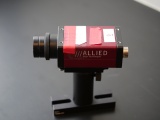
| + | <figure id="fig:Manta_camera_side_view"> | ||
| + | [[Image:Manta camera side view.jpeg|thumb|right|<caption>Side view of the Matna G-032 camera. The detector is recessed inside the body of the camera, 17.5 mm from the end of the housing. The detector comprises an array of 656x492 square pixels, 7.4 μm on a side. The active area of the detector is 4.85 mm (H) × 3.64 mm with a diagonal measurement of 6 mm. The manual for the camera is available online [https://www.1stvision.com/cameras/AVT/dataman/Manta_TechMan.pdf here].</caption>]] | ||
| + | </figure> | ||
| + | * When everything is set, measure the distance <math>S_o</math> from the target object to the lens and the distance <math>S_i</math> from the lens to the camera detector. | ||
| + | ** <xr id="fig:Manta_camera_side_view" /> shows the location of the detector inside of the camera. | ||
| + | * In the image acquisition window, press <tt>Acquire</tt> (lower right). | ||
| + | * Save your image to the MATLAB workspace | ||
| + | ** Your image is saved in <tt>foo.ImageData</tt> but it will be overwritten next time you acquire an image. You will need to copy the image into a new variable before continuing. | ||
| + | ** Return to the MATLAB console window. | ||
| + | ** Choose a descriptive variable name such as <tt>Image1</tt> and save your data to it: | ||
| + | <pre>Image1 = foo.ImageData;</pre> | ||
| + | * Compute the magnification. | ||
| + | ** In the MATLAB <tt>Command Window</tt>, display your image by typing <tt>figure; imagesc( Image1 ); colormap gray;</tt> | ||
| + | ** Go back to the command window (by pressing <tt>ALT</tt>-<tt>TAB</tt> on the keyboard or selecting it from the task bar) and type <tt>imdistline</tt>. | ||
| + | ** Use the line to measure a feature of known size on the micro ruler | ||
| + | *** The small tick marks are 10 μm apart | ||
| + | *** The large tick marks are 100 μm apart | ||
| + | *** The whole pattern is 1 mm long. | ||
| + | *** The pixel size is 7.4 μm | ||
| + | * Does your value agree with the ones predicted by the lens makers' formula? | ||
| + | |||
| + | ======Repeat for several image and object distances and plot the results====== | ||
| + | * Repeat the procedure at several image and object distances. Do an equal number with the target placed at less than and greater than 2<math>f</math> from the lens. | ||
| + | * Record your measurements | ||
| + | * Plot the results | ||
| + | ** Plot <math>{1 \over S_i}</math> as a function of <math> {1 \over f} - {1 \over S_o}</math>. | ||
| + | ** Plot <math>{h_i \over h_o}</math> as a function of <math>{S_i \over S_o}</math>. | ||
| + | * Do the relationships between <math>M</math>, <math>S_o</math>, and <math>S_i</math> match the theory? | ||
* What sources of error affect your measurements? | * What sources of error affect your measurements? | ||
| − | |||
| − | {{: | + | Don't take your apparatus apart just yet. You will use it in the next section. |
| + | |||
| + | ===Lab exercise 3: noise in images=== | ||
| + | Almost all measurements of the physical world suffer from some kind of noise. Capturing an image involves measuring light intensity at numerous locations in space. The [https://www.alliedvision.com/en/products/cameras/detail/Manta/G-032.html Manta G-032] CCD cameras in the lab measure about 320,000 unique locations for each image. Every one of those measurements is subject to noise. In this part of the lab, you will quantify the random noise in images made with the Manta cameras, which are the same ones that you will use in the microscopy lab. | ||
| + | |||
| + | <figure id="fig:Camera_noise_data"> | ||
| + | [[File:Noise experiment data.png|thumb|right|<caption>Noise measurement experiment. The cameras in the lab produce images with 656 horizontal by 492 vertical picture elements, or ''pixels''. At regular intervals, the camera measures the intensity of light falling on each pixel and returns an array of ''pixel values'' <math>P_{x,y}[t]</math>. The pixel values are in units of analog-digital units (ADU).</caption>]] | ||
| + | </figure> | ||
| + | So what is noise in an image? Imagine that you pointed a camera at a perfectly static scene — nothing at all is changing. Then you made a movie of, say, 100 frames without moving the camera or anything in the scene or changing the lighting at all. In this ideal scenario, you might expect that every frame of the movie would be exactly the same as all the others. <xr id="fig:Camera_noise_data"/> depicts a dataset generated by this thought experiment as a mathematical function <math>P_{x,y}[t]</math>. If there is no noise at all, the numerical value of each pixel in all 100 of the images would be the same in every frame: | ||
| + | |||
| + | :<math>P_{x,y}[t]=P_{x,y}[0]</math>, | ||
| + | |||
| + | where <math>P_{x,y}[t]</math> is the the ''pixel value'' reported by the camera of at pixel <math>x,y</math> in the frame that was captured at time <math>t</math>. The square braces indicated that <math>P_{x,y}</math> is a discrete-time function. It is only defined at certain values of time <math>t=n\tau</math>, where <math>n</math> is the frame number and <math>\tau</math> is the interval between frame captures. <math>\tau</math> is equal to the inverse of the ''frame rate'', which is the frequency at which the images were captured. | ||
| + | |||
| + | You probably can guess that IRL, the frames will not be perfectly identical. We will talk in class about why this is so. For now, let's just measure the phenomenon and see what we get. A good way to make the measurement is to go ahead and actually do our thought experiment: make a 100-frame movie of a static scene and then see how much each pixel varies over the course of the movie. Any variation in a particular pixel's value over time must be caused by random noise of one kind or another. Simple enough. | ||
| + | |||
| + | (An alternate way to do this experiment would be to simultaneously capture the same image in 100 identical, parallel universes. This will obviously reduce the time needed to acquire the data. You are welcome to use this alternative approach in the lab.) | ||
| + | |||
| + | <figure id="fig:Camera_noise_plot_axes"> | ||
| + | [[File:Camera noise plot axes.png|thumb|right|<caption>Pixel variance versus mean mystery plot. Can you stand the suspense?</caption>]] | ||
| + | </figure> | ||
| + | We need a quantitative measure of noise. ''Variance'' is a good, simple metric that specifies exactly how unsteady a quantity is, so let's use that. In case it's been a while, variance is defined as <math>\operatorname{Var}(P)=\langle(P-\bar{P})^2\rangle</math>. | ||
| + | |||
| + | So here's the plan: | ||
| + | |||
| + | * Point your camera at a static scene that has a range of light intensities from bright to dark. | ||
| + | * Make a movie. | ||
| + | * Compute the variance of each pixel over time. | ||
| + | * Make a scatter plot of each pixel's variance on the vertical axis versus its mean value on the horizontal axis, as shown in <xr id="fig:Camera_noise_plot_axes"/>. | ||
| + | |||
| + | Plotting the data this way will reveal whether or not the quantity of noise depends on intensity. With zero noise, the plot would be a horizontal line on the axis. But you know that's not going to happen. How do you think the plot will look? | ||
| + | |||
| + | ====Set up the scene and adjust the exposure time==== | ||
| + | The first step is to set up a scene with a large range of intensities. It's also important to measure roughly the same number of pixels for each intensity value. How can we diagnose the intensity range and number of pixels at each intensity? Enter the histogram. This useful plot will tell you the distribution of pixel intensities in your image. In our case, we will use a histogram to help us maximize the range and even out the number of pixels at each intensity. | ||
| + | |||
| + | For this part of the lab, you will change your experimental set up to obtain an image with an approximately uniform intensity histogram. Lucky for you, the <tt>UsefulImageAcquisition</tt> tool displays the intensity histogram of your image in the top right corner of the Image Acquisition window. It is up to you to decide how to get the best image, but here are a few guidelines: | ||
| + | |||
| + | <figure id="fig:Example_noise_setup_histogram"> | ||
| + | [[File:Example noise setup intensity histogram.png|thumb|right|<caption>Example intensity histogram with approximately uniform distribution of pixel values over the range 10-2000 ADU.</caption>]] | ||
| + | </figure> | ||
| + | * In the Image Acquisition window, click <tt>Start Preview</tt>. | ||
| + | * Set the <tt>Exposure</tt> property to 100. | ||
| + | * Adjust your experiment until your histogram is a roughly uniform distribution of pixel values between about 10 and 2000. <xr id="fig:Example_noise_setup_histogram"/> shows a reasonably nice histogram. You might want to try some combination of sliding the optical components around, and adjusting the exposure time and LED current (remember not to exceed 0.5A!). | ||
| + | * Make a schematic including relevant distances of your final setup. | ||
| + | |||
| + | If you ever want to plot your own histogram from a saved image, here is some example MATLAB code to do just that: | ||
| + | |||
| + | <pre> | ||
| + | [ counts, bins ] = hist( double( squeeze( exposureTest(:) ) ), 100); | ||
| + | semilogy( bins, counts, 'LineWidth', 3 ) | ||
| + | xlabel( 'Intensity (ADU)' ) | ||
| + | ylabel( 'Counts' ) | ||
| + | title( 'Image Intensity Histogram' ) | ||
| + | </pre> | ||
| + | |||
| + | If you're curious, the <tt>hist</tt> MATLAB function takes in the intensities you measured in the image <tt>exposureTest</tt>, divides the maximum range of intensities into a given number of equally spaced intervals or 'bins' (100 in this case), then counts the number of pixels which fall into each bin. | ||
| + | |||
| + | ====Acquire movie and plot results==== | ||
| + | Once you are set up correctly, make a movie and plot the results using the procedure below: | ||
| + | |||
| + | # Capture a 100 frame movie. | ||
| + | ## Go to the Image Acquisition window and change the <tt>Number of Frames</tt> property from 1 to 100. | ||
| + | ## Press <tt>Acquire</tt>. | ||
| + | ## Switch to the MATLAB console window. (Press <tt>alt</tt>-<tt>tab</tt> until the console appears.) | ||
| + | ## Save the movie to a variable called <tt>noiseMovie</tt> by typing: <tt> noiseMovie = foo.ImageData</tt>; | ||
| + | # Plot pixel variance versus mean. | ||
| + | ## Use the code below to make your plot. | ||
| + | |||
| + | <pre> | ||
| + | pixelMean = mean( double( squeeze( noiseMovie) ), 3 ); | ||
| + | pixelVariance = var( double( squeeze( noiseMovie) ), 0, 3 ); | ||
| + | [counts, binValues, binIndexes ] = histcounts( pixelMean(:), 250 ); | ||
| + | binnedVariances = accumarray( binIndexes(:), pixelVariance(:), [], @mean ); | ||
| + | binnedMeans = accumarray( binIndexes(:), pixelMean(:), [], @mean ); | ||
| + | figure | ||
| + | loglog( pixelMean(:), pixelVariance(:), 'x' ); | ||
| + | hold on | ||
| + | loglog( binnedMeans, binnedVariances, 'LineWidth', 3 ) | ||
| + | xlabel( 'Mean (ADU)' ) | ||
| + | ylabel( 'Variance (ADU^2)') | ||
| + | title( 'Image Noise Versus Intensity' ) | ||
| + | </pre> | ||
| + | |||
| + | (Need a refresher on loglog plots? [[Understanding log plots|Click here]].) | ||
| + | |||
| + | ====Questions==== | ||
| + | * Did the plot look the way you expected? | ||
| + | * How does noise vary as a function of light intensity? | ||
| + | * Include the plot in your writeup. | ||
| + | ** To save the MATLAB plot, Select File ... Save in the plot window | ||
| + | ** Select PNG format | ||
| + | *** Do not save plots in JPEG format. JPEG compression makes them difficult to read. | ||
| + | ** Name the file and save it | ||
| + | ====Don't forget to clean up==== | ||
| + | * Once you are done with the lab exercises, please disassemble your apparatus and return components to their homes. | ||
{{Template:20.309 bottom}} | {{Template:20.309 bottom}} | ||
Latest revision as of 20:09, 31 July 2017


Overview
You are going to build a microscope next week. The goal of the Optics Bootcamp exercise is to make that seem like a less intimidating task. The bootcamp mixes a little bit of mens and a little bit manus. It starts with a few written problems, followed by some exercises in the lab. The written problems will help you with the lab work. After you do the problems, come on by the lab. (Or do the problems in lab if you would like some help.) You will build an imaging apparatus made from some of the same optical components you will use in the microscopy lab, including an LED illuminator, an object with precisely spaced markings, a lens, and a CCD camera. You will compare measurements of object distance, image distance, and magnification to the values predicted by the lens makers' formula that was covered in class. You will also measure the noise characteristics of the CCD cameras we use in the lab.
For a good review of geometrical optics, ray tracing, and some worked-out ray tracing examples, see this page.
Problems
Problem 1: Snell's law
A laser beam shines on to a rectangular piece of glass of thickness $ T $ at an angle $ \theta $ of 45° from the surface normal, as shown in the diagram below. The index of refraction of the glass, ng, is 1.41 ≈√2. The index of refraction for air is 1.00.

(a) At what angle does the beam emerge from the back of the glass?
(b) When the beam emerges, in what direction (up or down) is it displaced?
Optional:
(c) By how much will the beam be displaced from its original axis of propagation?
Problem 2: chelonian size estimation
In the diagram below, an observer at height $ S $ above the surface of the water looks straight down at a turtle swimming in a pool. The turtle has length $ L $, height $ H $, and swims at depth $ D $.

(a) Use ray tracing and Snell's law to locate the image of the turtle. Show your work.
(b) Is the image real or virtual?
(c) Is the image of the turtle deeper, shallower, or the same depth as its true depth, $ D $?
(d) Is the image of the turtle longer, shorter, or the same length as its true length, $ L $?
(e) Is the image of the turtle taller, squatter, or the same height as its true height, $ H $?
Problem 3: ray tracing with thin, ideal lenses
Lenses L1 and L2 have focal lengths of f1 = 1 cm and f2 = 2 cm. The distance between the two lenses is 7 cm. Assume that the lenses are thin. The diagram is drawn to scale. (The gridlines are spaced at 0.5 cm.) Note: Feel free to print out this diagram so you can trace the rays directly onto it. Or maybe use one of those fancy tablet thingies that the kids seem to like so much these days.

(a) Use ray tracing to determine the location of the image. Indicate the location on the diagram.
(b) Is the image upright or inverted? Is the image real or virtual?
(c) What is the magnification of this system?
Optional:
(d) Lens L1 is made of BK7 glass with a refractive index n1 of 1.5. Lens L2 is made of fluorite glass with a refractive index n2 of 1.4. Compute the focal lengths of L1 and L2 if they are submerged in microscope oil (refractive index no = 1.5).
Problem 4: this will be really useful later
In the two-lens system shown in the figure below, the rectangle on the left represents an unspecified lens L1 of focal length $ f_1 $ separated by 0.5 cm from another lens L2 with focal length $ f_2 $ of 1 cm.

Find the value of $ f_1 $ such that all the rays incident parallel on this system will be focused at the observation plane, located at a distance d of 2 cm away from L2.
Lab orientation
Welcome to the '309 Lab. Before you get started, take a little time to learn your way around.


The 20.309 lab contains more than 15,000 optical, mechanical, and electronic components that you may choose from in order to complete your assignments throughout the semester. You can waste a lot of time looking for things, so take a little time to learn your way around. The floor plan below shows the layout of rooms 16-352 and 16-336. When you get to the lab, take a walk around, especially to the center cabinet, west cabinet, and west drawers. Go everywhere and check things out for a few minutes. Read the time machine poster near the printer. Discover the stunning Studley tool chest poster near the east parts cabinet.
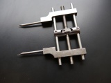
You probably noticed that many components are filed in boxes labeled with a sequence of letters and numbers. A company called Thorlabs manufactures the most of the optics and optical mounts you will use. The lab manuals frequently refer to components by their part number, which is usually one or two letters that have a vague relationship to the name of the part, followed by a couple of numbers. For example, the Thorlabs part number for a certain type of cage plate is "CP02." Thorlabs makes many kinds of cage plates, each with a subtle variation in its design. All of the cage plate part numbers starts with the letters "CP," followed by some numbers and in some cases a letter or two at the end. The Thorlabs website has an overview page of various kinds of cage plates here. Googling "Thorlabs CP02" is a quick way to get to the catalog page for that part.
To the untrained eye, many of the components in the lab are indistinguishable. The picture on the right shows just one example of strikingly-similar-looking bits. Take care when you select components from stock. Students sometimes return components to the wrong bins. Use even more care when you put things away. It is helpful to sing the One of These Things is Not Like the Others song from Sesame Street out loud while you are putting things away to ensure that you don't make any errors. (For the final exam, you will be required to identify various components while blindfolded.)

Note that Station 9 is now the "Instructor Station," and the previously labeled instructor station is now "Station 5" and available for your use.
See! Wasn't that a worthwhile journey?
Lab exercises
Lab exercise 1: measure focal length of lenses
Measure the focal length of the four lenses marked A, B, C, and D located near the lens measuring station.

Lab exercise 2: imaging with a lens
In this part of the lab, you are going to build a simple imaging system with one lens and compare measurements of the object distance $ S_o $, image distance $ S_i $, and magnification $ M $ with the values predicted by the lens makers' formula:
- $ {1 \over S_o} + {1 \over S_i} = {1 \over f} $
- $ M = {h_i \over h_o} = {S_i \over S_o} $

Figure 2 is a picture of the thing you are about to build. From left to right, the apparatus includes an illuminator, an object (a glass slide with a precision microruler pattern on it), an imaging lens, and a camera to capture images. All of the components are mounted in an optical cage made out of cage rods and cage plates. The cage plates are held up by optical posts inserted into post holders that are mounted on an optical table. You will be able to adjust the positions of the object and lens by sliding them along the cage rods.
Gather materials
You can spend a huge amount of time walking around the lab just getting things in the lab, so it makes sense to grab as many parts as possible in one trip. Figure 2 should give you some idea of what the parts look like.
The materials you will need for this lab are shown in the image gallery below, including a part number and descriptive name of each component. When you come across a part name or number that is not-all-that-self-explanatory, remember that google is your friend. Most of the parts are manufactured by a company called ThorLabs. If you ever have a question about any of the components, the ThorLabs website can be very helpful. For example, if the procedure calls for an SPW602 spanner wrench and you have no idea what such a thing might look like, try googling the term: "thorlabs SPW602". You will find your virtual self just a click or two away from a handsome photo and detailed specifications.

Screw sizes are specified as <diameter>-<thread pitch> x <length> <type>. The diameter specification is confusing. Diameters ¼" and larger are measured in fractional inches, whereas diameters smaller than ¼" are expressed as an integer number that is defined in the Unified Thread Standard. The thread pitch is measured in threads per inch, and the length of the screw is also measured in fractional inch units. So an example screw specification is: ¼-20 x 3/4. Watch this video to see how to use a screw gauge to measure screws. (There is a white, plastic screw gauge located near the screw bins.) The type tells you what kind of head the screw has on it. We mostly use stainless steel socket head cap screws (SHCS) and set screws. If you are unfamiliar with screw types, take a look at the main screw page on the McMaster-Carr website. Notice the useful about ... links on the left side of the page. Click these links for more information about screw sizes and attributes. This link will take you to an awesome chart of SHCS sizes.
Parts you will need for this lab:
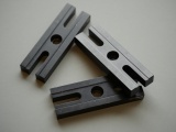
- Optical breadboard(Located in the lower left cubby of the Instructor Cubbies):
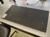
Optical breadboard

- Optomechanics (located in plastic bins on top of the center parts cabinet):
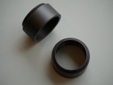
2 x 0.5" Lens tube (SM1L05)
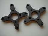
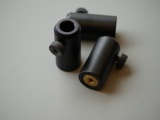
2 x 2" Cage plate (LCP01, looks like an "O" in a square)
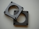
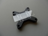
4 x Cage plate adapter (LCP02, looks like an "X")
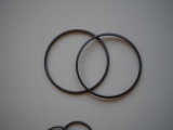
2 x 2" Retaining rings (SM2RR)


- Optomechanics (located on the counter above the west drawers):
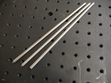
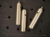
3 x ER8 cage assembly rod (The last digit of the part number is the length in inches.)
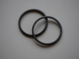
3 x 1" Retaining rings (SM1RR)


- Optics (located in the west drawers):
1 x LA1951 plano-convex, f = 25 mm lens (this will be used as a condenser for your illuminator)
1 x LB1811 biconvex, f = 35 mm lens (this will be used to form an image of your object)

- Screws and Posts (located on top of the west parts cabinet):
3 x Post holders (PH2)
3 x Optical posts (TR2)
3 x Mounting base (BA1)
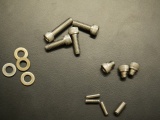
3 x 8-32 set screws,
3 x ¼-20 x 1/4" or socket head cap screws,
4 x ¼-20 x 3/4;" socket head cap screws,
1 x ¼-20 set screw,
4 washers


- More Parts (Located on top of the east cabinet):
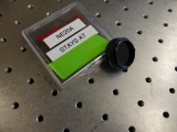
1 x ND filter
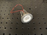
1 x red, super-bright LED (mounted in heatsink)
Microruler calibration slide mounted to a cage plate adapter


Most of the tools you will need are located in the drawers next to your lab station. Hex keys (also called Allen wrenches) are used to operate SHCSs. Some hex keys have a flat end and others have a ball on the end, called balldrivers. The ball makes it possible to use the driver at an angle to the screw axis, which is very useful in tight spaces. You can get things tighter (and tight things looser) with a flat driver. Here is a list of the tools you will need:
- Tools (located in your station's drawers):
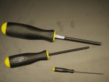
1 x 3/16 hex balldriver for 1/4-20 cap screws
1 x 9/64 hex balldriver,
1 x 0.050" hex balldriver for 4-40 set screws (tiny)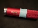
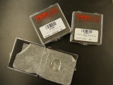
1 x SPW602 spanner wrench


You will also need to use an adjustable spanner wrench. The adjustable spanner resides at the lens cleaning station. There are only one or two of these in the lab. It is likely that one of your classmates neglected to return it to the proper place. This situation can frequently be remedied by yelling, "who has the adjustable spanner wrench?" at the top of your lungs. Try not to use any expletives. And please return the adjustable spanner wrench to the lens cleaning station when you are done.
1 x SPW801 adjustable spanner wrench

- Things that should already be (and stay at) your lab station:
1 x Manta CCD cameraballdriver for 4-40 set screws (tiny)
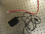
1 x Calrad 45-601 power adapter for CCD,
1 x ethernet cable connected to the lab station computer


Build the apparatus
Use the image of the apparatus to think about how to put your system together. The following guidelines should help get you started. If at any point you have questions, do not hesitate to ask an instructor for help.
Mount the LED


- Mount the LED between two SM2RR retaining rings in an LCP01 cage plate.
- Screw in one SM2RR to a depth of 1 mm.
- Run the wires of the LED through the opening in the LCP01 and insert the LED until it is resting on the retaining ring. It will get sandwiched in-between two retaining rings.
- Add a second SM2RR retaining ring to secure the LED. Use the SPW801 adjustable spanner wrench or a small flat bladed screwdriver to tighten the retaining ring. The SPW801 can be opened until its width matches the SM2RR diameter, the separation between the ring's notches.
- Screw a TR2 optical post into the threaded hole in the side of the LCP01 cage plate (holding the LED) using an 8-32 set screw.
- Use a ¼-20 x 1/4" SHCS to connect a BA1 mounting base to a PH2 post holder.
- Use a ¼-20 x 3/4" SHCS to secure the base to the optical breadboard. (You don't need to use two screws.)
- Insert the post into the holder and tighten the thumbscrew to fix its height.
Mount the lenses in lens tubes

- Place the 35 mm lens in a SM1L05 lens tube.
- Don't just drop the lens in. Use lens paper to gently lower the lens into the tube.
- The lens will rest against a ridge inside of the tube, near the threaded end.
- Don't touch the lens while you are putting it in.
- Start threading an SM1RR retaining ring into the tube and then tighten it with the red SPW602 spanner wrench.
- Thread an SM1RR retaining ring in another SM1L05 lens tube and use the SPW602 spanner wrench to drive it about 90% of the way down the tube.
- Place the 25 mm lens in a SM1L05 lens tube with its curved side facing the external threads of the lens tube.
- Thread a second SM1RR retaining ring into the lens tube and tighten it with the SPW602 spanner wrench.
Mount optical components on LCP02 cage plates

- Screw the lens tube with the 35 mm lens into a LCP02 cage plate (the one that looks like an X.)
- Screw the lens tube with the 25 mm lens a into another LCP02. Screw the ND filter into the other side of the LCP02.
Construct the cage

- Place three cage rods (ER8) through the holes in the LCP01 cage plate holding the LED so that their ends are flush with the plate.
- Secure the cage rods by tightening the 4-40 set screws (see picture).
- Slide the other cage plates on to the rods on your other cage plates in the correct order (25 mm lens/ND filter, object, 35mm lens).
- Secure the open end of the cage rods with another LCP01 cage plate mounted on an optical post and post holder.
- Slide this cage plate on so that about ½" of cage rod pokes out. This will give you room for another cage plate to go on. Tighten the setscrews.
- Add an LCP02 cage plate adapter to the end of the cage. Tighten the set screws of the final two cage plates.
Attach the camera
- The should already be mounted on a post and base. Put the tube that extends from the camera into the hole in the LCP02 cage plate at the end of your cage.
- Use a ¼-20 x 3/4" SHCS and a washer to secure the base and keep the camera from moving around.
This is not an ideal setup. The way the camera is attached to the cage is pretty cheesy. We'll give you a better way to do it in the microscopy lab.
Connect the LED


- Turn the power supply on.
- Make sure the power supply is not enabled (green LED below the OUTPUT button is not lit).
- Use the righthand set of knobs to set the current and voltage
- Adjust the CH1/MASTER VOLTAGE knob so the display reads about 5 Volts.
- Adjust the CH1/MASTER CURRENT knob to so the display reads 0.1 Amps.
- IMPORTANT: Never set the CURRENT to a value greater than 0.5A, as this will burn out the LED.
- Connect the + (red) terminal of channel CH1 on the power supply to the red wire of the LED.
- Connect the - (black) terminal of channel CH1 on the power supply to the black wire of the LED.
- Press the OUTPUT button to enable the power supply and light the LED.
- Adjust the LED brightness using the power supply's CURRENT knob.
Measure object and image distances; magnification
Adjust the lens and object
- Start with the object at about 2$ f $ = 70 mm from the lens.
- Launch MATLAB
- In the command window, start the image acquisition tool by running the following two lines of code:
foo = UsefulImageAcquisition;
foo.Initialize
- After the Image Acquisition window appears, click the Start Preview button.
- Set the exposure time
- In the lower right side of the window, edit Exposure to obtain a well-exposed image. The units are in microseconds.
- You can keep the default values for the Gain, Frame Rate, and Number of Frames for now.
- You may also need to adjust the current in your LED. Remember not to exceed 0.5 A.
- Move the lens and the object to produce a focused image.
Measure stuff

- When everything is set, measure the distance $ S_o $ from the target object to the lens and the distance $ S_i $ from the lens to the camera detector.
- Figure 4 shows the location of the detector inside of the camera.
- In the image acquisition window, press Acquire (lower right).
- Save your image to the MATLAB workspace
- Your image is saved in foo.ImageData but it will be overwritten next time you acquire an image. You will need to copy the image into a new variable before continuing.
- Return to the MATLAB console window.
- Choose a descriptive variable name such as Image1 and save your data to it:
Image1 = foo.ImageData;
- Compute the magnification.
- In the MATLAB Command Window, display your image by typing figure; imagesc( Image1 ); colormap gray;
- Go back to the command window (by pressing ALT-TAB on the keyboard or selecting it from the task bar) and type imdistline.
- Use the line to measure a feature of known size on the micro ruler
- The small tick marks are 10 μm apart
- The large tick marks are 100 μm apart
- The whole pattern is 1 mm long.
- The pixel size is 7.4 μm
- Does your value agree with the ones predicted by the lens makers' formula?
Repeat for several image and object distances and plot the results
- Repeat the procedure at several image and object distances. Do an equal number with the target placed at less than and greater than 2$ f $ from the lens.
- Record your measurements
- Plot the results
- Plot $ {1 \over S_i} $ as a function of $ {1 \over f} - {1 \over S_o} $.
- Plot $ {h_i \over h_o} $ as a function of $ {S_i \over S_o} $.
- Do the relationships between $ M $, $ S_o $, and $ S_i $ match the theory?
- What sources of error affect your measurements?
Don't take your apparatus apart just yet. You will use it in the next section.
Lab exercise 3: noise in images
Almost all measurements of the physical world suffer from some kind of noise. Capturing an image involves measuring light intensity at numerous locations in space. The Manta G-032 CCD cameras in the lab measure about 320,000 unique locations for each image. Every one of those measurements is subject to noise. In this part of the lab, you will quantify the random noise in images made with the Manta cameras, which are the same ones that you will use in the microscopy lab.

So what is noise in an image? Imagine that you pointed a camera at a perfectly static scene — nothing at all is changing. Then you made a movie of, say, 100 frames without moving the camera or anything in the scene or changing the lighting at all. In this ideal scenario, you might expect that every frame of the movie would be exactly the same as all the others. Figure 5 depicts a dataset generated by this thought experiment as a mathematical function $ P_{x,y}[t] $. If there is no noise at all, the numerical value of each pixel in all 100 of the images would be the same in every frame:
- $ P_{x,y}[t]=P_{x,y}[0] $,
where $ P_{x,y}[t] $ is the the pixel value reported by the camera of at pixel $ x,y $ in the frame that was captured at time $ t $. The square braces indicated that $ P_{x,y} $ is a discrete-time function. It is only defined at certain values of time $ t=n\tau $, where $ n $ is the frame number and $ \tau $ is the interval between frame captures. $ \tau $ is equal to the inverse of the frame rate, which is the frequency at which the images were captured.
You probably can guess that IRL, the frames will not be perfectly identical. We will talk in class about why this is so. For now, let's just measure the phenomenon and see what we get. A good way to make the measurement is to go ahead and actually do our thought experiment: make a 100-frame movie of a static scene and then see how much each pixel varies over the course of the movie. Any variation in a particular pixel's value over time must be caused by random noise of one kind or another. Simple enough.
(An alternate way to do this experiment would be to simultaneously capture the same image in 100 identical, parallel universes. This will obviously reduce the time needed to acquire the data. You are welcome to use this alternative approach in the lab.)

We need a quantitative measure of noise. Variance is a good, simple metric that specifies exactly how unsteady a quantity is, so let's use that. In case it's been a while, variance is defined as $ \operatorname{Var}(P)=\langle(P-\bar{P})^2\rangle $.
So here's the plan:
- Point your camera at a static scene that has a range of light intensities from bright to dark.
- Make a movie.
- Compute the variance of each pixel over time.
- Make a scatter plot of each pixel's variance on the vertical axis versus its mean value on the horizontal axis, as shown in Figure 6.
Plotting the data this way will reveal whether or not the quantity of noise depends on intensity. With zero noise, the plot would be a horizontal line on the axis. But you know that's not going to happen. How do you think the plot will look?
Set up the scene and adjust the exposure time
The first step is to set up a scene with a large range of intensities. It's also important to measure roughly the same number of pixels for each intensity value. How can we diagnose the intensity range and number of pixels at each intensity? Enter the histogram. This useful plot will tell you the distribution of pixel intensities in your image. In our case, we will use a histogram to help us maximize the range and even out the number of pixels at each intensity.
For this part of the lab, you will change your experimental set up to obtain an image with an approximately uniform intensity histogram. Lucky for you, the UsefulImageAcquisition tool displays the intensity histogram of your image in the top right corner of the Image Acquisition window. It is up to you to decide how to get the best image, but here are a few guidelines:

- In the Image Acquisition window, click Start Preview.
- Set the Exposure property to 100.
- Adjust your experiment until your histogram is a roughly uniform distribution of pixel values between about 10 and 2000. Figure 7 shows a reasonably nice histogram. You might want to try some combination of sliding the optical components around, and adjusting the exposure time and LED current (remember not to exceed 0.5A!).
- Make a schematic including relevant distances of your final setup.
If you ever want to plot your own histogram from a saved image, here is some example MATLAB code to do just that:
[ counts, bins ] = hist( double( squeeze( exposureTest(:) ) ), 100);
semilogy( bins, counts, 'LineWidth', 3 )
xlabel( 'Intensity (ADU)' )
ylabel( 'Counts' )
title( 'Image Intensity Histogram' )
If you're curious, the hist MATLAB function takes in the intensities you measured in the image exposureTest, divides the maximum range of intensities into a given number of equally spaced intervals or 'bins' (100 in this case), then counts the number of pixels which fall into each bin.
Acquire movie and plot results
Once you are set up correctly, make a movie and plot the results using the procedure below:
- Capture a 100 frame movie.
- Go to the Image Acquisition window and change the Number of Frames property from 1 to 100.
- Press Acquire.
- Switch to the MATLAB console window. (Press alt-tab until the console appears.)
- Save the movie to a variable called noiseMovie by typing: noiseMovie = foo.ImageData;
- Plot pixel variance versus mean.
- Use the code below to make your plot.
pixelMean = mean( double( squeeze( noiseMovie) ), 3 );
pixelVariance = var( double( squeeze( noiseMovie) ), 0, 3 );
[counts, binValues, binIndexes ] = histcounts( pixelMean(:), 250 );
binnedVariances = accumarray( binIndexes(:), pixelVariance(:), [], @mean );
binnedMeans = accumarray( binIndexes(:), pixelMean(:), [], @mean );
figure
loglog( pixelMean(:), pixelVariance(:), 'x' );
hold on
loglog( binnedMeans, binnedVariances, 'LineWidth', 3 )
xlabel( 'Mean (ADU)' )
ylabel( 'Variance (ADU^2)')
title( 'Image Noise Versus Intensity' )
(Need a refresher on loglog plots? Click here.)
Questions
- Did the plot look the way you expected?
- How does noise vary as a function of light intensity?
- Include the plot in your writeup.
- To save the MATLAB plot, Select File ... Save in the plot window
- Select PNG format
- Do not save plots in JPEG format. JPEG compression makes them difficult to read.
- Name the file and save it
Don't forget to clean up
- Once you are done with the lab exercises, please disassemble your apparatus and return components to their homes.