Difference between revisions of "Optical Microscopy Part 2: Fluorescence Microscopy"

Contextual Background

Recommended reading

• Lectures 1 through 9 of the 20.309 class

Design of a fluorescence microscope

Beam expansion

Similar triangles: the beam expands by the ratio of focal lengths, f2/f1

Your 20.309 microscope

20.309 microscope block diagram	20.309 student's microscope

Components in the 20.309 lab

Laser illumination and laser safety

The fluorescent illumination source is a 5 mW, λ=532 nm green laser.

Do not begin working with the laser until you are familiar with laser safety procedures. If you missed laser safety training, please see an instructor. Wear the correct laser safety eyewear at all times — even when your laser is not on — since other groups may be using theirs. Make sure the laser warning light outside the main door to the lab is flashing before you turn on a laser. Never point the laser toward other people. Laser light can emerge from the top of the objective lens. Never put your face directly above the objective.

Keep in mind these best practices when it comes to laser safety:

• Do not operate a laser unless the flashing laser warning sign is on.
• Wear safety goggles. Always check the marking on the goggles.
• Use the lowest possible power during alignment or adjustment. Use neutral density filters near the laser source.
• Know the beam path at all times.
• Keep your eyes out of the plane of the beam. This is normally a plane just above the optical table.
• Confine the beam inside lens tubes. As much as possible, fully enclose the laser beam path. Use a stop to prevent uncontained beams.
• Avoid stray rays. Keep your parts out of the beam path. Remove reflective clothing items, jewelry. Do not use reflective tools.
• Disable lasers when they are not in use. Remove a battery. Disconnect the power source.

Dichroic mirror and barrier filter

The fluorophores we use will emit light in the orange-red region of the visible spectrum (550-600 nm) when excited by the 532 nm green laser.

In any fluorescence system, a key concern is viewing only the emitted fluorescence photons, and eliminating any background light, especially from the illumination source. Two optical elements address the problem. A dichroic mirror reflects light of one wavelength, and passes light of another. The transmission spectrum for the 565DCXT from Chroma Technologies, which is similar to your NT47-268 dichroic from Edmund Optics, is shown in Figure 3. In contrast, a barrier filter blocks a particular spectral region extremely well. We will use the E590LPv2 barrier filter from Chroma Technologies.

The figure below shows the transmittance of the dichroic mirror and barrier filter over a range of wavelengths. The barrier filter is essential for high-sensitivity fluorescence imaging as it will block any reflected green light while allowing trace amount of red light from the fluorophores. It will also pass the red light from the LED in the illuminator for bright field imaging so that you can accomplish combined bright field and fluorescent imaging to help set up your sample.

The transmission spectra for the 565DCXT dichroic and the E590LPv2 barrier filter

Samples

You have the following samples available for imaging with both 40× and 100× objectives:

• A fluorescence reference slide
• Several types of sample slides with 4 μm or 1 μm red-fluorescent beads (several different dyes, but with peak excitation roughly 535nm, peak emission roughly 575nm)
• PSF slides with 100 nm or 190 nm red-fluorescent beads

Plot of an Airy function with Rayleigh resolution R=1, and a best-fit Gaussian function with σ=0.46869.

Data processing: Converting Gaussian fit to Rayleigh resolution

One method for measuring resolution is to fit a Gaussian function to an image of a very small source such as a fluorescent PSF microsphere. If the source is small enough, the image approximates the optical system's point spread function. As evidenced by the plot at right, the Gaussian function looks a lot like the central maximum of the Airy function.

The Rayleigh resolution of the Airy function shown is 1. The σ of the corresponding Gaussian is 0.46869. Thus, to convert the Gaussian fit to Rayliegh resolution, multiply σ by 1/0.46869 = 2.13361.

Note that some Gaussian fitting functions (such as gaussfit) return sqrt(2) * σ, instead of σ. In this case, multiply the value returned by 1/(sqrt(2) * 0.46869) = 1.50869. The occurs because the gaussfit function does not include the customary factor of two in its denominator. The equation implemented by gaussfit is:

F = (a(1) * exp(-((X - a(5)) .^ 2 / (a(2) ^ 2) + (Y-a(6)) .^ 2 / (a(3) ^ 2))) + a(4));

Here is the code that generated the plot:

xAxis = -10:0.01:10;

% generate an Airy disk profile with a normalized resolution R=1
firstBesselZero = 3.8317;
airyFunction = 2 * abs(besselj(1, firstBesselZero * xAxis)./ ...
               (firstBesselZero * xAxis));
airyFunction(xAxis == 0) = 1;

% use nonlinear regression to fit a Gaussian function to the Airy disk
gaussianFunction = @(parameters, xdata)  parameters(2) * ...
                   exp( -xdata .^ 2 / (2 * parameters(1) .^ 2) );

bestFitGaussianParameters = nlinfit(xAxis, airyFunction, gaussianFunction, [1 1]);
lsqcurvefit(gaussianFunction, [1 1], xAxis, airyFunction);
bestFitGaussian = gaussianFunction(bestFitGaussianParameters, xAxis);
sigma = bestFitGaussianParameters(1);
sigmaToFwhmConversionFactor = 2 * sqrt(2*log(2));
fwhm = sigmaToFwhmConversionFactor * sigma;

% plot the results
plot(xAxis, airyFunction);
hold on;
plot(xAxis, bestFitGaussian, 'r');
title(texlabel(['Airy Function (R=1) versus ...
      Gaussian (sigma = ' num2str(sigma) ' FWHM = ' num2str(fwhm) ')']));

Instructions

Microscope construction

Place holders and mounts for all components

• Verify your design with one of the lab instructors before proceeding with construction.
• Remember: Verify focal length and cleanliness of all your lenses before adding them to your microscope.
• Prepare the mounting tubes for L3, L4, and L5 such that they can slide along their guiding struts. Note the difference between the (0.35" thick) CP02 cage plates (for L3, L4, and L5) and the thicker (0.5" thick) CP02T cage plate. Use the latter sparingly, where a non-threaded junction of the mounting struts is needed.
• Place the dichroic mirror DM on a cube optic mount (B5C), affix the mount on a kinematic plate (B4C) and in the cage cube (C4W).
  • Ask an instructor for help if you need to clean a dichroic mirror or barrier filter. (These optics have exposed coatings and must be cleaned with extra care.)
  • 

    

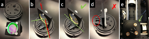    Dichroic mirror mount
  • (a) The soft clear screws affix the dichroic mirror without deforming nor scratching its surface. No "slipping and scratching"! Be utterly vigilant and steady as you handle the screwdriver.
  • (b) Green light will be reflected by the dichroic mirror, while red light will be transmitted through. When handling a thick dichroic mirror, to ascertain which surface is the reflecting green one, watch the reflection of a soft object (e.g. paper) as it touches the mirror: on the green surface, the image will appear to be touching the object; on the other side, source and image will appear to be a few millimeters apart.
  • (c) and (d) Making sure the green reflecting surface of the dichroic mirror is exactly on a diameter of the kinematic stage. (Otherwise pre-DM alignment will be totally lost post-DM!). The mounting bracket should not stand in the way of the rotation of the kinematic stage; this motion will be crucial to the microscope's alignment.
  • (e) Use soft black screws, only moderately tightened down, to hold the kinematic stage into the cage cube.

Alignment of the fluorescence illumination light

• Start with no L3, L4, L5 nor objective lenses between the laser source and the sample stage. Adjust the laser position as well as the M2 and M3 mirror orientation (via their two knobs) to center the excitation light path. Insert a neutral density filter (ND filter) between the laser and M2 to dim the beam power. You can use adjustable "target" pinholes / adjustable irises to gauge beam alignment both on its horizontal and its vertical trajectories.

Using pinholes and irises to optimize initial microscope alignment

• Next, add the beam expander. Fine-tune the distance separating L3 and L4 to optimize beam collimation at the sample stage level. Again, strive for best alignment through the pinholes.
  • Beam expansion criteria - Collimated light comes out of the laser pointer. The light should also be collimated when it reaches the sample (Kohler illumination). In order to provide a good image, the laser light should illuminate most of the field of view. The beam emerging from the laser pointer (approximately 1.1 mm) may not be wide enough. This means that the laser beam will need to be expanded. The design of the beam expander is a tradeoff. Overexpansion will decrease the light intensity at the sample and may not give you enough power for imaging. Underexpansion will result in very uneven illumination. What expansion factor should you use for a 40× objective?
• Finally, add L5 and the 10× objective lens. Fine-tune the position of L5 for best beam collimation, as well as the orientation of M2, M3 and DM for best beam centering. How will the position of L5 change when you switch to the 40× and the 100× objective?

Barrier filter incorporation

To easily switch back and forth between bright-field and fluorescence microscopy mode, you may need to remove and add the barrier filter (BF) from your setup (this is obviously true and mandatory if your bright-field light source is a blue LED, whose transmitted light would otherwise be blocked by the E590LPv2 BF; the latter only transmits light of wavelength > 590 nm).

• Keeping in mind that barrier filters are designed to work under collimated light illumination, where do you intend to position the BF in your microscope light path?
• What wavelengths must your BF transmit?
• The barrier filter removes any light from the illumination laser that was not reflected by the dichroic mirror.
• Ask an instructor for help if you need to clean a dichroic mirror or barrier filter. (These optics have exposed coatings and must be cleaned with extra care.)
• During fluorescent imaging, you will not use the bright field illuminator. Bright-field capability is useful for first visualizing the sample and viewing what features are in the field of view. Your design should retain the ability to do both white light and fluorescent visualization.

Fluorescence Imaging

1. Use a fluorescence reference slide to center the field of view and to optimize the uniformity of illumination. Take an image of this, with both the 40× and 100× objectives. Use the histogram display of the camera software (function imhist in Matlab) to be certain that the image is not overexposed and that you are using the full dynamic range of the camera.
2. Under each magnification configuration (40× or 100×), take an image of the 4 μm and 1 μm red-fluorescent beads. Perform flat-field correction on the image (i.e. divide the image by a normalized copy of your reference image). Be sure that your microscope is in the same state when you record the reference image and the bead image. [Note: Actively enable the 12-bit option of the camera software, which otherwise defaults to 8-bit imaging]. Compare what you see before and after flat field correction.
3. Make initial images of the PSF slide. This slide consists of 190nm fluorescent beads, which are proxies for ideal point sources. The image of a practical point source object will closely approximate the ideal Airy disk. Calculate the approximate resolution of your microscope, using this measured Airy disk or Gaussian image (depending on the quality of your microscope and the resolution of the camera).

Example images:

Example images included by past students in their Part 2 report: (top) Fluorescent beads, (center) Fluorescence reference slide, (bottom) Histogram of camera pixel exposure distribution

Report: Microscope construction and fluorescence characterization

Microscope design

• Update the block diagram description of your microscope, its photograph, and annotation of pertinent optical components and distances.

Fluorescence imaging characterization

Demonstrate the epi-fluorescence imaging capability of your enhanced microscope:

• Provide the fluorescent reference image you collected with both the 40× and 100× objectives, as either an image (see imshow command in Matlab) or a surface plot (see surf command in Matlab), as well as a cross-section of signal intensity across its diagonal (see improfile command in Matlab).
• Exhibit your images of the 4 μm and 1 μm fluorescent bead samples, with both the 40× and 100× objectives. Compare and contrast these pictures before and after flat-field correction to counteract nonuniform illumination.
• Describe your flat-field correction procedure, from recording the reference image through applying the correction.
• Also provide log(y) scaled histograms of at least one original and corrected image pair.

Discussion on design and image quality

• Comment on your corrections and relate your results to your choices during beam expander design and construction.
• How do these choices relate to your intended experiments in weeks three and beyond?

Lab manual homepage

Lab Manual: Optical Microscopy