Estimating second order system parameters from noise power spectra using nonlinear regression

… the safe use of regression requires a good deal of thought and a good dose of skepticism

—Arnold Barnett

If your program generates an error message rather than curve fitting results, you probably won’t be able to make sense of the exact wording of the message.

—Motulsky and Shristopoulos. Fitting Models to Biological Data using Linear and Nonlinear Regression

You won't find a tool with more power per inch than a chain saw. Power like that requires extra attention to safety.

—lowes.com

A chainsaw masterpiece in process.

Overview

In the limits of detection lab, you will use regression to estimate the parameters of second order system models of the optical trap and atomic force microscope (AFM). MATLAB includes a powerful nonlinear regression function called nlinfit. Think of nlinfit like a chainsaw. Sharp power tools like nlinfit and chainsaws must be used with extraordinary care. In skilled hands, both of these productive and useful tools deliver sublime results. Inattentive or unskilled operation, on the other hand, engenders distorted, ugly, or even catastrophic outcomes.

Chainsaw accidents are graphic and obvious. Unfortunately, many serious regression mishaps present themselves more like mosquito bites or bruises than severed limbs. You can suffer a serious regression injury without even realizing it. Bad regressions can easily masquerade as good ones — concealing their insidious flaws behind a lovely, plausible pair of overlapping curves. Because of this, it especially important to maintain a critical and alert mindset in the vicinity of regression.

Another challenge of regression is that there are many indications of possible problems, but no definitive indicators to inform you that things have gone well. Its hard to know when it's safe to stop.

This page offers some advice that will help you retain all of your digits and limbs when you regress. In the spirit of of the gruesome car crash videos your high-school gym teacher forced you to watch in drivers' ed., several tragic regressions are illustrated along with pointers help you steer clear of pitfalls that lead to misfortune.

Remain vigilant at all times when you regress.

Regression concepts review

Nonlinear regression is a method for finding the relationship between a dependent variable $ y_n $ and an independent variable $ x_n $. The two quantities are related by a model function $ f(\beta, x_n) $. $ \beta $ is a vector of model parameters. The dependent variable $ y_n $ is measured in the presence of random noise, which is represented mathematically by a random variable $ \epsilon_n $. In equation form:

$ y_n=f(\beta, x_n)+\epsilon_n $.

The goal of regression is to determine a set of best-fit set of model parameters $ \hat{\beta} $ that match the observed data as closely as possible. Because the dependent variable includes noise, $ \hat{\beta} $ will not be equal to $ \beta $. As you can probably guess, decreasing the noise or increasing the number of observations tends to make the difference between $ \hat{\beta} $ and $ \beta $ smaller.

Ordinary nonlinear least squares regression assumes that:

• the independent variable is known exactly, with zero noise,
• the error values are independent and are all values of $ \epsilon_n $ are drawn from the same distribution (i.i.d),
• the distribution of the error terms has a mean value of zero,
• the independent variable covers a range adequate to define all the model parameters, and
• the model function exactly relates $ x $ and $ y $.

These assumptions are almost never perfectly met in practice. It is important to consider how badly the regression assumptions have been violated when assessing results.

Get ready …

You need four things to run a regression:

1. a vector containing the values of the independent variable;
2. a vector containing the corresponding observed values of the dependent variable;
3. a model function; and
4. a vector of initial guesses for the model parameters.

Power spectrum of x-axis QPD voltage. 3.2 μm silica spheres trapped with 80 mW laser power. Sampling frequency was 50 MHz.

Independent variable and observations

The second order system model of the optical trap makes predictions about the power spectrum of a thermally excited, trapped microsphere, whereas the instrument actually records a time sequence of voltages from the QPD position detector. The raw data must be converted into a power spectrum before fitting.

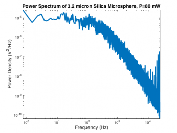
MATLAB has a function called pwelch that computes a power spectrum $ P_{xx}(f) $ and associated frequency bin vector $ f $ from a time series. Like many MATLAB functions, there are several different ways to invoke pwelch. Even judging by Mathworks' low standards for clarity and consistency, the various forms of pwelch are perplexing. Here is the command that generated the spectrum on the right:

[ Pxx, frequency ] = pwelch( OpticalTrapTimeDataX, [], [], [], 50000 );

The first argument, OpticalTrapTimeDataX is an Nx1 vector containing the QPD x-axis voltage samples. Empty values for the next three parameters (window, noverlap, and f) leave them set to their default values. The last argument is the sampling frequency, $ f_s $. We will reexamine the default parameter settings later on.

In order to make the best choice of independent and dependent variables, it is necessary to consider the relative influence of measurement noise on the two quantities in the regression: frequency and power density. The optical trap has a very accurate and precise oscillator circuit that generates its sample clock. This high-quality timebase allows frequencies in the QPD signal to be determined with almost no error. Power density, on the other hand, is inherently noisy due to constant perturbation of the trapped particle's position by the random thermal driving force. You can see how wiggly the power spectrum is in the vertical direction.

It's an easy choice: frequency will serve as the independent variable in the regression and power density will be the dependent variable.

Model function

nlinfit requires that the regression model be expressed as a function that takes two arguments and returns a single vector of predicted values. The signature of the model function must must have the form:

[ PredictedValues ] = ModelFunction( Beta, X ).

The first argument is a vector of model parameters. The second argument is a vector of independent variable values. The return value must must have the same size as the second argument.

The MATLAB function below models the power spectrum of a second-order system excited by white noise. The three model parameters are passed to the function in a 1x3 vector: undamped natural frequency $ f_0 $, damping ratio $ \zeta $, and low-frequency power density $ P_0 $.

function [ PowerDensity ] = SecondOrderSystemPowerSpectrum( ModelParameters, Frequency )
    
    undampedNaturalFrequency = 2 * pi * ModelParameters(1);
    dampingRatio = ModelParameters(2);
    lowFrequencyPowerDensity = ModelParameters(3);

    s = 2i * pi * Frequency;

    response = lowFrequencyPowerDensity * undampedNaturalFrequency.^2 ./ ...
        ( s.^2 + 2 * undampedNaturalFrequency * dampingRatio * s + undampedNaturalFrequency.^2 );
    
    PowerDensity = abs( response ).^2;

end

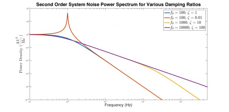
It's a good idea to test the model function out before you use it. The plot below shows the output of SecondOrderSystemPowerSpectrum for three sets of parameter values and a frequency vector that goes from 10 Hz to 25 KHz. It's comforting to see that the curves have the expected shape.

Model power spectra of critically damped, underdamped, and overdamped second order systems excited by white noise. The underdamped response is flat at low frequencies, exhibits a narrow peak near $ f_0 $, and decreases with slope -4 at high frequencies. The critically damped response is flat from low frequency until approximately $ f_0 $, after which it falls with a slope of -4. Both overdamped systems are flat at low frequencies. They decrease with slope -2 at intermediate frequencies from approximately $ \frac{f_0}{\zeta} $ to $ f_0 $, after which the response falls with slope -4.

Initial guesses

nlinfit infers the number of model parameters from the size of the Initial guess vector. Accordingly, the initial guesses should be stored in a 1x3 vector. You can eyeball a reasonable starting point by taking a look at the PSD plot, say: 500 Hz for $ f_0 $, 10^-5 AU²/Hz for $ P_0 $, and 1 for the damping ratio.

Get set …

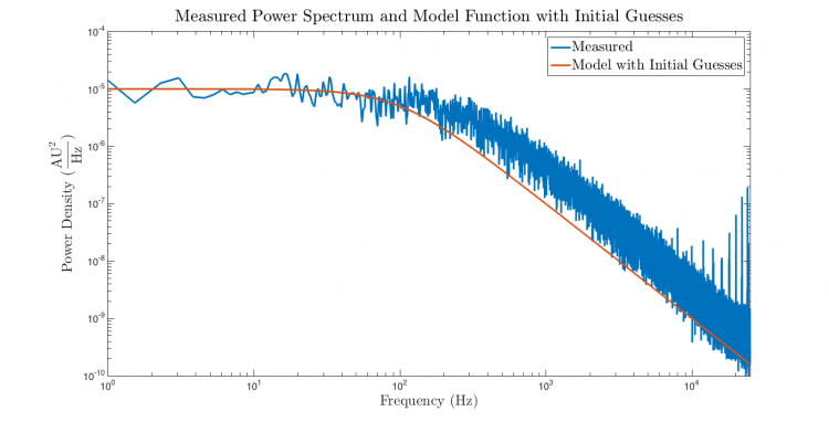
The first step of all regressions is to plot the observations and the model function evaluated with the initial guesses versus the independent variable on a single set of axes. Don't attempt to run nlinfit until you've done this plot. It is much easier to ensure that the arguments to nlinfit are in order before you regress than to debug a screen full of cryptic, red text. Side effects of premature regression include confusion, waste of time, fatigue, irritability, alopecia, and feelings of frustration. There is no chance that nlinfit will succeed if there is a problem with one of its arguments.

Go ahead ... do the plot.

The plot looks good enough to proceed.

Go ... first attempt

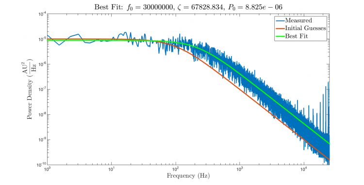
Here are the results of running nlinfit with the data, model, and initial guesses developed so far:

Success! Great curves!

Not so fast. If you let the alluring, overlapping blue and green curves in the plot above get you excited, go back and reread this page from the beginning. Much more scrutiny is required. On top of the usual reasons to be skeptical, an additional cause for concern materialized in the console output window. MATLAB barfed up a long, impenetrable, red word salad of foreboding verbiage:

Warning: Some columns of the Jacobian are effectively zero at the solution, indicating that 
the model is insensitive to some of its parameters.  That may be because those parameters 
are not present in the model, or otherwise do not affect the predicted values.  It may also be 
due to numerical underflow in the model function, which can sometimes be avoided by choosing 
better initial parameter values, or by rescaling or recentering.  Parameter estimates may be 
unreliable. 
> In nlinfit (line 373)

William Shatner in Nick of Time.

This unavailing communiqué is so perfectly unclear that it's impossible to know how to react. Deep concern? Annoyance? Fear? Rage? Apathy? (It's just a warning, after all.) We will come back to the warning later. For now, you will have to take it on faith that red text spewing from nlinfit is never good news, but it is sometimes not bad news. This time, the root cause of the warning is serious and fundamental. Unfortunately, none of the clues offered in the text point toward the real source of the problem, and some of the suggestions offered are downright misleading.

When it comes to error messages and warnings, nlinfit works just like the Mystic Seer that featured prominently in the unforgettable 43rd Twilight Zone episode Nick of Time starring William Shatner as a superstitious newlywed with car trouble and Patricia Breslin as his sensible bride. Over-interpreting the intentionally vague pronouncements of a mechanical contrivance can get you into all kinds of trouble. The real enemy is inside. Or is it?

Get out of town while you still can.

Assessing the regression 1: examine the residuals

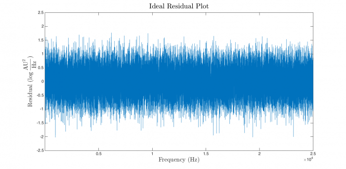
Violations of the regression assumptions are a leading cause of trouble. After every regression, do the responsible thing: spend some time ascertaining how disgraceful the sin you just committed was. A good first step is to plot the residuals and have a look at them. (The second value returned from nlinfit contains a vector of the residuals.) If the regression assumptions are perfectly met, the plot should look something like this:

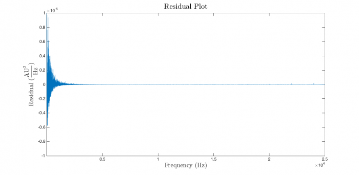
It's easy to convince yourself that the residuals in the plot above are independent and identically distributed. Compare that to the residual plot for the current regression:

Red Alert! The residual plot doesn't bear even cursory scrutiny. The magnitude of the residuals decreases dramatically as frequency increases — a significant and unacceptable violation of the regression assumptions. We definitely have a bad regression on our hands.

This has to be fixed before moving on.

Attempt #2

The biggest issue with the first regression attempt is that the assumed distribution of the error terms was not a good model for the actual measurement noise. In retrospect, this problem should have been obvious. A quick glance at the PSD plot reveals that the measurement error (fuzziness of the line) is about the same size at all frequencies. But the plot axes are scaled logarithmically. A certain level of fuzziness near the top of the plot represents a much larger error magnitude than the same amount of fuzziness near the bottom of the plot. The error magnitude is not even close to constant, so there wan't much hope of getting a good residual plot.

Feel free to skip the next paragraph. It offers a hand-waving motivation for why the magnitude of the error in power density is not the same for all frequencies. This is not a mathematically precise argument. If you want to see some equations, take a look at this presentation as a starting point.

The magnitude dependence of measurement error in a noise power spectrum is an inherent feature of this type of measurement. Think about it this way … (handwaving alert); The measurement model consists of an input signal (white noise) that is transformed by a (second order) system. Over an infinite time period, the spectrum of input white noise signal is perfectly flat. But over a finite period, this is not true. White noise is stochastic, so by pure chance there will be a little more of some frequencies in a finite-time window and a little less of others. For obvious reasons, the optical trap's power spectrum was not measured over an infinite time period. During the interval that the QPD voltage was measured, the input power spectrum was not perfectly flat. This noisy input power spectrum got multiplied by the magnitude squared of the optical trap's transfer function. Assuming the distribution of noise magnitude started out equal at all frequencies, the measurement error in the output power spectrum is thus proportional to the magnitude squared of the power density.

Multiplicative error is a much better model of the measurement error in the noise power spectrum than the additive noise assumed by the regression model. Fortunately, there are a few easy ways to fix the problem. One approach is to transform the dataset into log space:

$ \log{y_n}=\log{f(\beta,x_n)\epsilon_n}=\log{f(\beta,x_n)}+log{\epsilon_n} $

Taking the log of the dependent variable turns multiplicative noise into additive noise. The code below uses MATLAB's anonymous function syntax to create a log-space model function.

logModelFunction = @( p, f ) log( SecondOrderSystemPowerSpectrum( p, f ) );

Simple enough. Now call nlinfit with logModelFunction instead of @ModelFunction. Remember to also take the log of $ P_{xx} $.

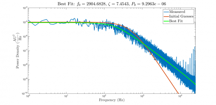
Here are the results:

Note that the estimate of $ f_0 $ changed by more than 250 Hz.

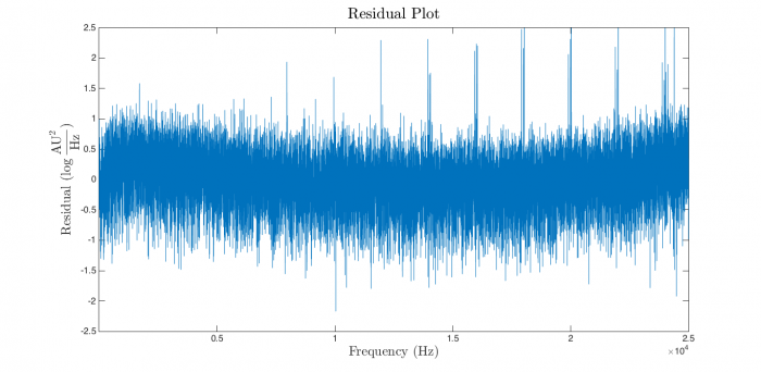
And the residual plot:

The residual plot is much closer to the ideal. There is a slight smile shape to the curve that indicates the presence of some systematic error in the model. (The model function does not perfectly match the system — perhaps due to nonlinearity.) But the distribution of the residuals looks a great deal more like the ideal plot and the deviation from the model is small.

MATLAB's warning this time is much shorter (but not more helpful):

Warning: The Jacobian at the solution is ill-conditioned, and some model parameters may not be
estimated well (they are not identifiable).  Use caution in making predictions. 
> In nlinfit (line 376) 

In general, the less red text produced by nlinfit the better. Progress.

Assessing the regression take 2: parameter confidence intervals

Range of independent variable

Power spectra of critically damped, underdamped, and overdamped second order systems excited by white noise. The underdamped response is flat at low frequencies, exhibits a narrow peak near $ f_0 $, and decreases with slope -4 at high frequencies. The critically damped response is flat from low frequency until approximately $ f_0 $, after which it falls with a slope of -4. Both overdamped systems are flat at low frequencies. They decrease with slope -2 at intermediate frequencies from approximately $ \frac{f_0}{\zeta} $ to $ f_0 $, after which the response decreases with slope -4.

Comparing the three regressions