Difference between revisions of "Estimating second order system parameters from noise power spectra using nonlinear regression"
(→Model function) |
(→Model function) |
||
| Line 46: | Line 46: | ||
===Model function=== | ===Model function=== | ||
<pre> | <pre> | ||
| − | function [ Magnitude | + | function [ Magnitude ] = SecondOrderSystemResponse( ModelParameters, Frequency ) |
undampedNaturalFrequency = ModelParameters(1); | undampedNaturalFrequency = ModelParameters(1); | ||
| Line 58: | Line 58: | ||
Magnitude = abs( response ); | Magnitude = abs( response ); | ||
| − | |||
end | end | ||
Revision as of 12:53, 25 May 2015
… the safe use of regression requires a good deal of thought and a good dose of skepticism
Overview
In the limits of detection lab, you will use regression to estimate the parameters of second order system models of the optical trap and AFM. MATLAB includes a powerful nonlinear regression function called nlinfit. Like all sharp tools, nlinfit must be used with extreme care. Regression is a delicate business.
Many common regression missteps spawn subtle errors rather than catastrophic failures. Because of this, bad regressions easily masquerade as good ones — hiding their insidious flaws behind a lovely, plausible pair of overlapping curves. This page illustrates several flawed regressions with the hope of helping you navigate the concealed hazards of fitting power spectra.
Remain vigilant at all times when you regress.
Regression review
Nonlinear regression is a method for finding the relationship between a dependent variable $ y_n $ and an independent variable $ x_n $. The two quantities are related by a model function $ f(\beta, x_n) $. $ \beta $ is a vector of model parameters. $ y_n $ is measured in the presence of random noise, which is represented mathematically by a random variable $ \epsilon_n $. In equation form:
$ y_n=f(\beta, x_n)+\epsilon_n $.
The goal of regression is to find the set of model parameters $ \hat{\beta} $ that best matches the observed data.
Ordinary nonlinear least squares regression assumes that:
- the error terms have a mean value of zero,
- the error terms are independent and identically distributed (i.i.d.),
- the independent variable is known exactly, with zero noise, and
- the independent variable covers a range adequate to define all the model parameters.
These assumptions are almost never perfectly met in practice. It is important to consider how badly these assumptions have been violated when evaluating the results of a regression.
Get ready …
You need four things to run a regression:
- a vector containing the values of the independent variable;
- a vector containing the corresponding observed values of the dependent variable;
- a model function; and
- a vector of initial guesses for the parameters.
Power spectrum
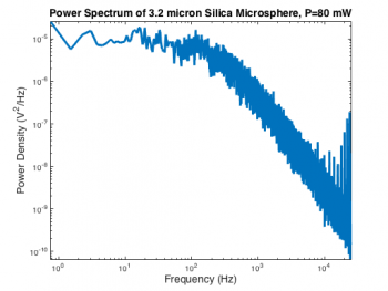
The optical trap records a sequence of voltages from the QPD, sampled at frequency $ f_s $. In the regression for the limits of detection lab, frequency, $ f $, is the independent variable, and power, $ P_{xx} $ is the dependent variable. The time series must be transformed into a power spectrum. An example power spectrum from the optical trap is shown on the right.
The MATLAB function pwelch computes a power spectrum and associated frequency vector from a time series. Like many MATLAB functions, pwelch can be called with different sets of parameters. The signatures of pwelch are particularly opaque — even by Mathworks' standards. Here is the command that generated the example spectrum above:
[ Pxx, frequency ] = pwelch( OpticalTrapTimeDataX, [], [], [], 50000 );
The first argument, OpticalTrapTimeDataX is an Nx1 vector containing the QPD x-axis voltage samples. Empty values for the next three parameters (window, noverlap, and f) leave them set to their default values. We will reexamine these parameters later on. The last parameter, 50000, is the sampling frequency.
Model function
function [ Magnitude ] = SecondOrderSystemResponse( ModelParameters, Frequency )

    undampedNaturalFrequency = ModelParameters(1);
    dampingRatio = ModelParameters(2);
    dcGain = ModelParameters(3);

    s = 2i * pi * Frequency;

    response = dcGain * undampedNaturalFrequency.^2 ./ ...
        ( s.^2 + 2 * undampedNaturalFrequency * dampingRatio * s + undampedNaturalFrequency.^2 );

    Magnitude = abs( response );

end
signature [ PredictedValues ] = ModelFunction( Beta, x)
First attempt
Range of independent variable
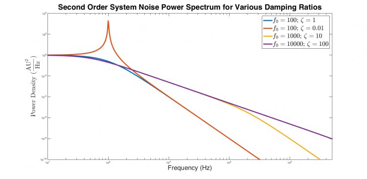
| Power spectra of critically damped, underdamped, and overdamped second order systems excited by white noise. The underdamped response is flat at low frequencies, exhibits a narrow peak near $ f_0 $, and decreases with slope -4 at high frequencies. The critically damped response is flat from low frequency until approximately $ f_0 $, after which it falls with a slope of -4. Both overdamped systems are flat at low frequencies. They decrease with slope -2 at intermediate frequencies from approximately $ \frac{f_0}{\zeta} $ to $ f_0 $, after which the response decreases with slope -4. |


