Bode plots and frequency response

Overview

Only two things can happen to a sine wave passing through a linear, time-invariant system: it's magnitude can be changed; and the signal can be delayed. The delay and percentage change in the magnitude are a function of frequency. A transfer function, H(f), is a complex-valued function of frequency that specifies the magnitude and phase shift of a particular system for all frequencies. The change in amplitude is often called the gain, and the delay is usually thought of in terms of a phase shift of the sine wave.

One way to visualize a transfer function is to make two plots. The first plot shows the gain verses frequency on a set of log-log axes. The second plot shows the phase shift versus log frequency. (Traditionally, Bode plots are constructed only using straight-line segments to represent the transfer function by means of straight edges and fine draft pen sets. Since plotting complicated functions is now done by computer, exact plots may be substituted for the traditional methods.)

First-order R-C low-pass filter.

Frequency response of common filters

Plot of low-pass filter with cutoff frequency $ f_C=1 $.

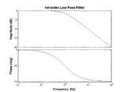
For example, consider a simple RC low-pass filter with the transfer function is given by

$ H(f) = \frac{V_{out}}{V_{in}} = \frac{1}{1 + j2\pi f RC} $

In this case the cutoff frequency is given by $ f_C = 1 / (2\pi RC) $. Several key features should be noted in the transfer function plot. For frequencies below $ f_C $, the gain is nearly flat (in this case at 1 or 0dB). For frequencies above $ f_C $, the gain drops off by a factor of 10 for each decade in frequency (expressed here in dB as -20dB/decade). At low frequency, the phase starts out at 0°, but starts to decrease noticeably at about $ f_C $/10, drops to -45° at $ f=f_C $, and asymptotes at -90° above 10×$ f_C $.

More examples

High-pass transfer function with cutoff frequency $ f_{HP}=1 $.

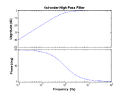
High-pass

$ H(f) = \frac{j f / f_{\rm HP}}{1 + j f / f_{\rm HP}} $

Second order low-pass transfer function. Note that the scale of the plots are double that of the 1st-order filter.

Second-order low-pass

$ H(f) = \left(\frac{1}{1 + j f / f_{\rm LP}}\right)^2 $

Frequency response of band-pass transfer function with $ f_{HP}=0.1 $ and $ f_{LP}=10 $.

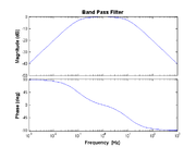
Band pass

$ H(f) = \frac{j f / f_{\rm HP}}{1 + j f / f_{\rm HP}} \times \frac{1}{1 + j f / f_{\rm LP}} $

MATLAB code

The transfer function plots were generated by the Matlab script wikibodeplots.m.