Difference between revisions of "Bode plots and frequency response"
Eliot Frank (Talk | contribs) |
|||
| Line 4: | Line 4: | ||
One way to visualize a transfer function is to make two plots. The first plot shows the gain verses frequency on a set of log-log axes. The second plot shows the phase shift versus log frequency. | One way to visualize a transfer function is to make two plots. The first plot shows the gain verses frequency on a set of log-log axes. The second plot shows the phase shift versus log frequency. | ||
| − | |||
| − | |||
[[Image:ElectronicsModuleFig-RC.png|thumb|right|First-order R-C low-pass filter.]] | [[Image:ElectronicsModuleFig-RC.png|thumb|right|First-order R-C low-pass filter.]] | ||
| Line 11: | Line 9: | ||
: <math> H(f) = \frac{V_{out}}{V_{in}} = \frac{1}{1 + j2\pi f RC} </math> | : <math> H(f) = \frac{V_{out}}{V_{in}} = \frac{1}{1 + j2\pi f RC} </math> | ||
| + | In this case the cutoff frequency is given by <math>f_C = 1 / (2\pi RC) </math>. | ||
| − | |||
| − | [[Image:BodePlot-LowPass.png|thumb|right|Bode plot of low-pass | + | [[Image:BodePlot-LowPass.png|thumb|right|Bode plot of low-pass filter with cutoff frequency <math> f_C=1 </math>.]] |
More examples | More examples | ||
| + | [[Image:BodePlot-HighPass.png|thumb|right|Bode plot of high-pass transfer function with cutoff frequency <math> f_{HP}=1 </math>.]] | ||
High-pass | High-pass | ||
| − | |||
: <math> H(f) = \frac{j f / f_{\rm HP}}{1 + j f / f_{\rm HP}} </math> | : <math> H(f) = \frac{j f / f_{\rm HP}}{1 + j f / f_{\rm HP}} </math> | ||
| + | [[Image:BodePlot-SecondOrder.png|thumb|right|Second order low-pass transfer function. Note that the scale of the plots are double that of the 1st-order filter.]] | ||
Second-order low-pass | Second-order low-pass | ||
| − | |||
: <math> H(f) = \left(\frac{1}{1 + j f / f_{\rm LP}}\right)^2 </math> | : <math> H(f) = \left(\frac{1}{1 + j f / f_{\rm LP}}\right)^2 </math> | ||
| + | [[Image:BodePlot-BandPass.png|thumb|right|Frequency response of band-pass transfer function with <math> f_{HP}=0.1 </math> and <math> f_{LP}=10 </math>.]] | ||
Band pass | Band pass | ||
| − | |||
| − | |||
: <math> H(f) = \frac{j f / f_{\rm HP}}{1 + j f / f_{\rm HP}} | : <math> H(f) = \frac{j f / f_{\rm HP}}{1 + j f / f_{\rm HP}} | ||
\times \frac{1}{1 + j f / f_{\rm LP}} </math> | \times \frac{1}{1 + j f / f_{\rm LP}} </math> | ||
{{Template:20.309 bottom}} | {{Template:20.309 bottom}} | ||
Revision as of 14:39, 3 April 2013
Overview
Only two things can happen to a sine wave passing through a linear, time-invariant system: it's magnitude can be changed; and the signal can be delayed. The delay and percentage change in the magnitude are a function of frequency. A transfer function, H(f), is a complex-valued function of frequency that specifies the magnitude and phase shift of a particular system for all frequencies. The change in amplitude is often called the gain, and the delay is usually thought of in terms of a phase shift of the sine wave.
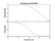
One way to visualize a transfer function is to make two plots. The first plot shows the gain verses frequency on a set of log-log axes. The second plot shows the phase shift versus log frequency.
For example, consider a simple RC low-pass filter with the transfer function is given by
- $ H(f) = \frac{V_{out}}{V_{in}} = \frac{1}{1 + j2\pi f RC} $
In this case the cutoff frequency is given by $ f_C = 1 / (2\pi RC) $.
More examples
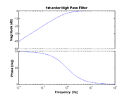
High-pass
- $ H(f) = \frac{j f / f_{\rm HP}}{1 + j f / f_{\rm HP}} $
Second-order low-pass
- $ H(f) = \left(\frac{1}{1 + j f / f_{\rm LP}}\right)^2 $
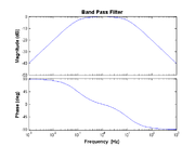
Band pass
- $ H(f) = \frac{j f / f_{\rm HP}}{1 + j f / f_{\rm HP}} \times \frac{1}{1 + j f / f_{\rm LP}} $


