Difference between revisions of "Assignment 8, Part 0: convolution practice"
From Course Wiki
MAXINE JONAS (Talk | contribs) |
Juliesutton (Talk | contribs) |
||
| Line 1: | Line 1: | ||
| + | <noinclude> | ||
[[Category:20.309]] | [[Category:20.309]] | ||
[[Category:Lab Manuals]] | [[Category:Lab Manuals]] | ||
[[Category:DNA Melting Lab]] | [[Category:DNA Melting Lab]] | ||
{{Template:20.309}} | {{Template:20.309}} | ||
| − | + | </noinclude> | |
| + | |||
{{Template:Assignment Turn In|message=Turn in your answers to the following questions}} | {{Template:Assignment Turn In|message=Turn in your answers to the following questions}} | ||
| Line 42: | Line 44: | ||
</ol> | </ol> | ||
| − | + | ||
| + | <noinclude> | ||
{{Template:Assignment 8 flow channel & two-color microscope navigation}} | {{Template:Assignment 8 flow channel & two-color microscope navigation}} | ||
{{Template:20.309 bottom}} | {{Template:20.309 bottom}} | ||
| + | </noinclude> | ||
Revision as of 14:32, 20 April 2020

| |
Turn in your answers to the following questions |
You may find the Fourier transform Tables 8.0.1 and 8.0.2 useful. Note that there are a few functions that you may not have seen before including:
- u(t) is the unit step function $ u(t) = \begin{cases} 0, & \text{if }t<0 \\ 1, & \text{if }t\geq0 \end{cases} $
- sinc(ax) is defined as: $ \text{sinc}(ax) = \frac{\sin(ax)}{ax} $
- rect(ax) is the box function: $ \text{rect}(ax) = \begin{cases} 0, & \text{if } |ax|> 1/2 \\ 1, & \text{if } |ax| \leq 1/2 \end{cases} $
- In class we found the Fourier transform of $ \cos^2(\omega_0 t) $. Use graphical convolution to determine the transform of $ \cos^4(\omega_0 t) $.
- Using the transform pairs in table 8.0.2, sketch the fourier transform of $ e^{-\alpha t} u(t) \times \cos(\omega_0 t) $. Assume that $ \alpha\ll\omega_0 $.
- Table 8.0.3 shows plots of eight time-domain signals A-H. The table on the right includes magnitude plots of the Fourier transform of ten signals numbered 1-10. For each time domain signal A-H, write the number 1-10 in the empty column of the matching frequency-domain signal. You may use a numbered plot more than once.
Some of the frequency plots are shown on log-log axes and some are linear, as indicated by the plot title.
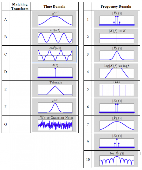

Table 8.0.3

- Overview
- Part 1: feedback systems
- Part 2: fabricate a microfluidic device
- Part 3: add flow control and test your device
Back to 20.309 Main Page