Difference between revisions of "20.109(S14):Preparing cells for analysis (Day4)"
MAXINE JONAS (Talk | contribs) m (8 revisions: Transfer 20.109(S14) to HostGator) |
|||
| (25 intermediate revisions by 4 users not shown) | |||
| Line 2: | Line 2: | ||
<div style="padding: 10px; width: 640px; border: 5px solid #FF6600;"> | <div style="padding: 10px; width: 640px; border: 5px solid #FF6600;"> | ||
| − | |||
| − | |||
| − | |||
| − | |||
==Introduction== | ==Introduction== | ||
| − | |||
| − | |||
| − | |||
| − | + | Today you will start collecting the key data for your chondrocyte or stem cell phenotype experiment. Recall that chondrocytes may de-differentiate to fibroblasts if not kept in the appropriate environment, while stem cells can undergo chondrogenesis under the right conditions. So, how do we tell chondrocytic and non-chondrocytic cell types apart? | |
| − | + | ||
| − | + | ||
| − | + | ||
| − | + | ||
| − | + | ||
| − | + | ||
| − | + | ||
| − | + | [[Image:20.109_cartilage.png|right|300px]] | |
| − | + | Folks trying to engineer cartilage tissue have been interested in this and similar questions for some time. After all, the more closely an ''in vitro'' or ''in vivo'' model construct can mimic natural tissue and promote its development, the more successful it may be for wound and disease repair. Engineering tissue thus requires an expert understanding of what the native tissue is like. Articular cartilage is a water-swollen protein network consisting of >50% collagen Type II, along with small amounts of collagen Types IX and XI. The collagen fibrils vary in diameter, cross-linking density, and orientation (random or aligned) depending on the depth of the tissue cross-section that is examined (see figure). Unlike cartilage, many other connective tissues are composed primarily of collagen Type I. | |
| − | + | ||
| − | + | ||
| − | + | ||
| − | + | ||
| − | + | Extracellular matrix (ECM) proteins such as the collagens must be synthesized by cells. Chondrocytes readily synthesize collagen II, while fibroblasts and mesenchymal stem cells primarily synthesize collagen I. Thus, both the expression and the production of different collagens is one way to distinguish these cell types. | |
| − | + | To study collagen at the gene transcript level, you will break open and homogenize your cells using a lysis reagent and column (the ominously named QIAshredder), and then isolate RNA using an RNeasy kit from Qiagen. The RNeasy kit includes silica gel columns, similar to the ones you used to purify DNA in Modules 1 and 2, that selectively bind RNA (but not DNA) that is >200 bp long under appropriate buffer conditions. Due to size exclusion but the porous beads, the resultant RNA is somewhat enriched in mRNAs relative to rRNAs and tRNAs. To further purify for mRNA, one could use a polyT affinity column to capture the polyA tail of this RNA type, but we will not do this step today. | |
| + | <br style="clear:both;"/> | ||
| − | + | After eluting and measuring your total RNA, you will perform a reverse transcription (RT) reaction to copy cDNA from the mRNA. Next time you will amplify the gene transcripts of interest, namely those for the collagen I and collagen II alpha chains, by PCR. In early iterations of this module, we used a one-step RT-PCR kit, and then ran the amplified cDNA products out on an agarose gel to compare the changes in collagen II and I expression for the two culture conditions. However, as you may have noticed by now, agarose gels do not have a large dynamic range. Moreover, end-point PCR is prone to error should the conditions – such as the amount of template RNA & ndash; deviate from those used to optimize the assay. For these reasons, we now use a more sensitive method for quantifying the transcripts, called real-time-PCR or sometimes RT-PCR, confusingly! The method is also called qPCR, for quantitative PCR. | |
| − | + | In qPCR, the amount of DNA is measured after ''each'' cycle of PCR, in contrast to an end-point PCR assay. The DNA is detected by using a dye that fluoresces only when it binds to DNA (similarly to ethidium bromide staining), or even a tagged primer that fluoresces only when it binds to the correct region of the template. As the DNA is amplified, fluorescence is repeatedly measured as it increases exponentially over time. Finally, cDNA product renaturing competes with primer annealing and the fluorescence intensity plateaus rather than growing. Comparisons between samples must be performed using data in the exponential regime. | |
| − | + | ||
| − | + | For both qPCR and end-point RT-PCR, housekeeping genes are used for normalization in order to compare transcript levels from different samples. Housekeeping genes are ones that are not expected to be affected by the experimental condition, such as essential genes for metabolism. To perform normalized end-point gel analysis, one simultaneously amplifies the cDNA of interest and a cDNA for a gene such as GAPDH in the same reaction tube. Primers are designed such that the two product sizes are distinguishable on a gel. To perform normalized qPCR, multiple primer sets can only be used in the same reaction if they are compatible with two different fluorophores. In our case, we will use a non-specific DNA stain that cannot distinguish different products, so we will run our experiment and control in separate wells. (The housekeeping gene that we will use is the gene encoding 18S ribosomal RNA, a concept that should be familiar from Module 1.) This experimental set-up means that your pipetting should be more careful than ever! | |
| − | For | + | [[Image: 20.109_RT-primers.png|right|325px]] |
| + | When measuring changes in gene expression, primer design must be appropriate for amplifying cDNA rather than genomic DNA. For example, a single primer that includes sequence from two neighboring exons, along with a second primer that has sequence from just one exon, will amplify mRNA but not genomic DNA – which may be present as a contaminant (see also figure at right). ''What would happen if each primer was complementary to sequence from only '''one''' exon?'' Primer design and quality control for qPCR also entail further consideration compared to bog standard PCR, particularly if tagged primers are used. In our case, the true efficiency of the primers needed to be measured in pilot experiments to enable later quantification of transcript level changes. Note that maximum primer efficiency is 2.0, i.e., perfectly exponential growth, while our primers range from about 1.7 to 1.9-fold increase per cycle. You will learn more about qPCR analysis in the coming week. | ||
| − | + | Next time (Day 5) we’ll initiate an assay called ELISA to observe collagen at the protein (rather than transcript) level and also begin analysis of the data collected thus far. | |
| − | + | ==Protocols== | |
| − | + | <font color=purple>If you got to go to the TC room first on Day 2, you will go in the second cohort today (and vice-versa). If you are in the second group, you may use the time that you are waiting to work on your FNT or the optional data analysis, but also be sure to prepare your RNase-free area, label tubes that you will need, etc., before heading into TC.</font color> | |
| − | + | ===Part 1: Prepare cell lysates=== | |
| − | + | You will prepare cell-bead samples in three different ways: one will allow you to count your cells, and is suitable for RNA preparation, while the other two will involve more stringent bead/matrix dissolution for better protein or proteoglycan recovery. Split up the work with your partner whatever way is most convenient. '''Remember to label your samples carefully at every step.''' | |
| − | + | ||
| − | + | ||
| − | + | ||
| − | + | <font color=FF33FF>'''If your beads are small and/or fragile, you may need to skip some rinsing steps today. Please also ask the teaching faculty for advice on working with your beads.'''</font color> | |
| − | + | #Before proceeding, briefly observe the cell-bead constructs under the microscope and note any changes from Day 3. | |
| + | #*Let the teaching faculty know if you have difficulty focusing within a bead. | ||
| + | #Remove the culture medium from each of your samples. Be careful not to suck up the beads; it will help to use a serological pipet just as you did when washing your freshly synthesized beads. Tipping the plate will help the beads settle in a cluster and allow you to remove medium elsewhere. | ||
| + | #*A 5 mL pipet size should work well for rigid beads, while for more delicate beads, you should use a 2 mL serological pipet or even a P1000. If your beads are falling apart, you can transfer the beads according to steps 3-5 below without trying to remove medium first. | ||
| + | #*If you are concerned about your bead amount, talk to the teaching faculty. You might skip the proteoglycan assay and focus on the other two instead.[[Image:S14_M3D4-overview.png|thumb|left|300px|'''Bead preparation for three assays.''']] | ||
| + | #About 1/3 of your beads will be used to measure protein content: move these to an eppendorf tube. The goal is about 10-15 (2-3 mm) beads per tube. | ||
| + | #*For large beads (4-5 mm), you might use only 5-10 beads, and for very small beads (<1 mm), you might use 20 or more. | ||
| + | #Another 1/3 will be used to measure proteoglycan content; these whole beads can also be moved to an eppendorf tube. | ||
| + | #The final 1/3 will be used to isolate RNA. Using a sterile spatula, transfer the beads into a fresh well of your 6-well plate. This transfer step is to exclude any cells that are growing on the bottom of the plate (as opposed to actually in the beads) from analysis. | ||
| − | + | ====Samples for RNA Isolation==== | |
| − | + | #Rinse the transferred bead-cell constructs with 4 mL of warm PBS, then aspirate the buffer. | |
| − | + | #*If your beads are very fragile, you might want to skip the PBS rinse, and directly proceed to step 2. | |
| − | # | + | #Add 3 mL of pre-warmed EDTA-citrate buffer, and incubate at 37 °C for 10 min. |
| − | # | + | #*Meanwhile, prepare the beads for the protein and proteoglycan assays as described below. '''All the materials that you need are in eppendorf tubes in the fridge.''' |
| − | # | + | #Now recover your cells: |
| − | # | + | #*Add 3 mL of warm complete culture medium, pipet up and down to break up the beads (you may find this easier with a 1 mL pipetman rather than a serological pipet), and transfer to a 15 mL conical tube. |
| − | # | + | #*Spin the cells down at 1900g for 6 min using the centrifuge that is in the TC room. |
| − | # | + | #Resuspend in ~ 1-1.5 mL of culture medium, and ''write down'' what you use. Mix thoroughly by pipetting, then set aside a 20 μL aliquot of your cells for counting, and put the rest of the cells into another eppendorf tube. |
| − | + | #*If you have very few cells based on your Day 3 observations and/or having very few beads, you might consider skipping the cell count, and instead keeping all of the cells for RNA isolation. If you have too few cells to get a reliable cell count, you are not losing valuable information for your report in any case. And if you have so few cells that taking some of them for a count compromises your other data, then that outcome would not be preferable to missing the cell count. | |
| − | + | #While one of you begins the spin in the main lab (see Part 2), the other should count your cell aliquot similarly to how you did on Day 2. This time, mix 10 μL of Trypan blue with your 20 μL of cells rather than using 90 μL, so we can conserve cells. '''Separately''' calculate the approximate numbers of live (yellowish) and of dead (blue) cells. | |
| − | + | #*Recall that you must multiply by 10,000 (and your dilution factor) to convert a hemacytometer cell count to a live cells/mL concentration. | |
| − | + | ||
| − | # | + | |
| − | # | + | |
| − | === | + | ====Samples for Protein Extraction==== |
| − | + | #Per eppendorf tube (typically 10-15 beads), add 133 μL of '''cold''' EDTA-citrate buffer (not from the warm conical!), and pipet up and down for 20-30 seconds to dissolve the beads. Be thorough while limiting bubbles as best you can. The resulting solution may be viscous. | |
| + | #Pipet 33 μL of 0.25 M acetic acid into each eppendorf tube. | ||
| + | #Finally, pipet 33 μL of 1 mg/mL pepsin (in 50 mM acetic acid) into each tube and mix well. | ||
| + | #Move your eppendorf tubes into the rack in the 4 °C fridge. Tomorrow the teaching faculty will move them to an elastase solution (also at 4 °C) to break down the polymeric collagen to more readily measured monomeric collagen. | ||
| − | + | ====Samples for Proteoglycan Extraction==== | |
| − | + | #Soak your beads for a few minutes in pre-warmed PBS, and then remove as much of the PBS as possible. Shoot to have as little pink tint to the beads as possible, as it is known to interfere with the proteoglycan assay. Repeat the soak step a second time with fresh PBS, if it seems to help. | |
| − | + | #Add 250 μL of papain solution to your beads. The papain is in an EDTA-citrate buffer base. | |
| − | + | #When the first partner goes to the main lab, s/he should take this tube to the 60 °C heat block. After 24 hours, the samples will be moved to the freezer. | |
| − | + | ||
| − | + | ||
| − | + | ===Part 2: RNA isolation and measurement=== | |
| − | + | Because you are preparing RNA, you will have to take special precautions during this part. RNA is strikingly different from DNA in its stability. Consequently it is more difficult to work with RNA in the lab. It is not the techniques themselves that are difficult; indeed, many of the manipulations are nearly identical to those used for DNA. However, RNA is rapidly and easily degraded by RNases that exist everywhere. There are several rules for working with RNA. They will improve your chances of success. Please follow them all. | |
| + | *Use warm water on a paper towel to wash lab equipment, such as microfuges, before you begin your experiment. Then wipe them down with “RNase-away” solution. | ||
| + | *Wear gloves when you are touching anything that will touch your RNA. | ||
| + | *Change your gloves often. | ||
| + | *Before you begin your experiment, clean and prepare your work area: (1) remove all clutter, (2) wipe down the benchtop with warm water and “RNase-away,” and (3) lay down a fresh piece of benchpaper and/or mark off the area with tape. This last step serves as a reminder to always wear your gloves when touching items in that area. | ||
| + | *Use RNA-dedicated solutions and if possible RNA-dedicated pipetmen. | ||
| + | *Get a new box of pipet tips from the RNA materials area and label their lid “RNase FREE” if the lid is not yet labeled. | ||
| − | == | + | #Pellet the cells for RNA isolation back in the main lab (8 min at 500 g). |
| − | + | #Remove the supernatant from your cell pellets using pipet tips from an RNase free tip box. | |
| − | * | + | #*Discard this and other supernatants in a conical waste tube. As you may remember from Module 1, the lysis reagent you will use shortly is not compatible with bleach. |
| − | * | + | #Now, in the fume hood, add 350 μL RLT with β-mercaptoethanol to each cell sample – vortex or pipet to mix. |
| − | * | + | #*If you have more than 5 million cells, you will need to double the amount of RLT used - talk to the teaching faculty. |
| + | #Add each cell lysate to a separate QIAshredder column, which is used to remove particulate matter. Microfuge the columns (over a 2 mL collection tube) for 2 min at max speed. '''Save the flowthrough!!!''' | ||
| + | #Add 1 volume (slightly > 350 μL) of 70% ethanol to each lysate and pipet to mix. | ||
| + | #Apply each sample (including any precipitate) to a separate RNeasy mini column (over a tube). Microfuge for 15 sec and discard the flowthrough. | ||
| + | #Add 700 μL RW1 buffer to each column. Microfuge 15 sec and discard the eluant again. | ||
| + | #Add 500 μL RPE buffer atop the columns, microfuge as before (15 sec), and discard the flowthrough. | ||
| + | #Repeat the addition of 500 μL RPE, but this time centrifuge for 2 min. prior to discarding the flowthrough. | ||
| + | #Transfer the columns to fresh 2 mL collection tubes. | ||
| + | #Centrifuge the column/tube "dry" for 1 min. Running a column like this helps to fully dry it, and to prevent carryover of ethanol. | ||
| + | #Trim the caps off of two new 1.5 ml eppendorf tubes (save the caps!) and label the sides of the tubes. | ||
| + | #Transfer the dried columns into the trimmed eppendorf tubes and elute the RNA from the columns by adding 30 μL of RNase-free water to each. Microfuge for 1 min, then cap the tubes and store the eluants on ice. | ||
| + | #Measure the concentration of your RNA samples. First prepare dilutions: 15 μL of of each in 385 μL sterile water. (The water does not strictly speaking have to be RNase-free since the RNA can be degraded and still give legitimate readings in the spectrophotometer.) | ||
| + | #This time you will work in "wavelength scan" mode on the spectrophotometer, rather than take readings only at 260 and 280 nm, as you may learn something about your samples from the shape of the entire curve from 250-290 nm. | ||
| + | #Begin with the cuvette containing blanking solution, and hit ''Blank'' on the spectrophotometer. | ||
| + | #Proceed to take an absorbance scan of each RNA sample. Record the 260 nm and 280 nm absorbance values in your notebook. You can simply touch your finger to the onscreen spectrum for coarse wavelength selection, and then touch the onscreen arrows for fine selection. | ||
| + | #Note the RNA concentrations of your samples in the table below, using the fact that 40 μg/mL of RNA will give a reading of A<sub>260</sub> = 1. Also calculate the 260:280 ratio, which should approach 2.0 for very pure RNA. | ||
| + | #Ideally, you will use 500 ng of RNA in each RT reaction. However, it's also useful to have all reactions to start with an equal amount of RNA template. (Although we will normalize with GAPDH transcripts, the more similar the samples are to begin with, the better.) At most you can use 7.5 μL of RNA per reaction. If you can use 500 ng per reaction within the above contraints, do so. Otherwise, figure out which one of your samples is limiting, and scale the other added sample amount so they are equal. If one sample is very low, or even below the detection limit of the spectrophotometer, don't scale to it and risk getting no data from either sample. Finally, note that if you use less than 7.5 μL RNA, water should be added to make up the difference. The table below may be helpful as you carry out your calculations. | ||
| + | |||
| + | <center> | ||
| + | {| border="1" | ||
| + | ! Sample | ||
| + | ! A<sub>260</sub> | ||
| + | ! Measured RNA conc. (μg/mL) | ||
| + | ! RNA conc. of undiluted stock (μg/mL) | ||
| + | ! Max RNA per rxn (ng in 7.5 μL) | ||
| + | ! Volume RNA needed per rxn | ||
| + | ! Volume water needed per rxn | ||
| + | |- | ||
| + | | 1: | ||
| + | | | ||
| + | | | ||
| + | | | ||
| + | | | ||
| + | | | ||
| + | | | ||
| + | |- | ||
| + | | 2: | ||
| + | | | ||
| + | | | ||
| + | | | ||
| + | | | ||
| + | | | ||
| + | | | ||
| + | |} | ||
| + | </center> | ||
| + | |||
| + | ===Part 3: RT reactions=== | ||
| + | |||
| + | #Set up your reactions on a cold block as usual. You will prepare one reaction for each of your samples. Random hexamer primers will be used so that all (we hope) transcripts are amplified. This approach is more convenient than adding unique primers for each transcript of interest. | ||
| + | #From one of the shared stocks, pipet 22.5 μL of RT master mix into each of two well-labeled PCR tubes. The master mix contains water, buffer, dNTPS, primers, and reverse transcriptase. | ||
| + | #Now you can add 7.5 μL of the appropriate RNA (or RNA and water as needed) to each tube. | ||
| + | #The following thermal cycler program will be used: 20 min at 25 °C, 30 min at 42 °C (reverse transcription step), and then cooling. After the RT is completed, the teaching faculty will store the samples in the freezer until next time. | ||
| + | |||
| + | <font color=purple>In whatever time remains today, you can continue work on your FNT or on the Module 3 mini-report. The steps to analyze your cell viability images are outlined below.</font color> | ||
| + | |||
| + | ===Part 4: Begin viability analysis (optional)=== | ||
| + | |||
| + | Starting today or as late as Day 6, you will use an image analysis program called ImageJ to quantify your live/dead data. This program is offered free of charge by the NIH (National Institutes of Health). | ||
| + | |||
| + | =====Cell Counting===== | ||
| + | |||
| + | Your goal for this section will be to compare the effort required for, and the resulting accuracy of, manually counting live and dead cells vs. doing so by semi-automated image analysis. After you are done, you might consider under what conditions you might prefer one method or the other. | ||
| + | |||
| + | If you don't have many cells to look at, extra data is available on today's [[Talk:20.109%28S13%29:Preparing_cells_for_analysis_%28Day4%29 | Talk]] page. | ||
| + | |||
| + | #Open your live cell image (green filter) by selecting ''File'' → ''Open'' | ||
| + | #Choose the line tool, and draw a line across the diameter of a typical cell | ||
| + | #Select ''Analyze'' → ''Set Scale'', and put 10 μm in under '''Known Distance''' | ||
| + | #*note: in lieu of using the exact pixel information from the camera, we simply are putting in the average size of a cell | ||
| + | #Convert your image to grey scale using ''Image'' → ''Type'' → ''8-bit'' | ||
| + | #Now you must somehow select your cells out from the background | ||
| + | #*One way to do this is by choosing ''Process'' → ''Binary'' → ''Make Binary''. However, you might find that clusters of cells are ‘read’ as a single cell. | ||
| + | #*An improved method is to use'' Image'' → ''Adjust'' → ''Threshold''. You can set the upper- and lower-bound intensities that define objects in your image. Play with the intensity sliders until your cells are mostly filled in with a red colour, but not overlapping with other cells whenever possible. | ||
| + | #Now you can count the objects. Choose ''Analyze'' → ''Analyze Particles'', and select ''Show'' →''Outlines'', ''Display Results'', ''Summarize'', and ''Record Stats''. Also choose a reasonable '''area''' (not diameter!) range for objects that are cell-sized. | ||
| + | #Try to play around with this process for a bit – are there any further changes you can make so the automated algorithm is as good as your eye? | ||
| + | #Record your final results (manual and best automated) in your notebook, for each sample that you have data for. Don’t forget to also manually count the dead cells, and subtract this number from the live cells (since the filter we used shows both green and red cells at once). | ||
| + | |||
| + | =====Statistical Analysis===== | ||
| + | |||
| + | Once you have cell counts (whether automated or manual) that you are happy with, you can do some basic statistical analysis. Isn't it nice to have way fewer samples than in Module 2? | ||
| + | |||
| + | #If you like, you may again download the linked [[Media: S09_20109_M2D5-Stats.xls | '''Excel file''']] as a framework to carry out the basic statistical manipulations below. The file is modified from one originally written by [http://web.mit.edu/be/people/engelward.htm Professor Bevin Engelward]. | ||
| + | #Find and plot 95% confidence intervals for the live cell counts and/or live cell percentage for each of your two samples. | ||
| + | #*What are the advantages and disadvantages of looking at counts versus percentages? In what situations would looking at counts be misleading? | ||
| + | #Compare the means (count and/or percentage) of your two samples. At what confidence level (if any) are they different? | ||
==For next time== | ==For next time== | ||
| − | + | #Write a brief response (250 ± 50 words) to one of the excerpts that were handed out in lecture and lab. | |
| + | #*These excerpts are drawn (with some editing) from previous 20.109 student essays about the prospect of standardization in tissue engineering. | ||
| + | #*You may revise the response you started during lecture, or write a brand new one. | ||
| + | #*Due on M3D5 (one week from today). | ||
| + | #[[20.109(S14):Module 3 oral presentations| '''The primary assignment''']] for this experimental module will be for you to develop a research proposal and present your idea to the class. For next time, please describe five recent findings that might define an interesting research question. You should hand in a 3-5 sentence description of each topic – in your own words – and cite an associated reference from the scientific literature. The topics you pick can be related to any aspect of the class, i.e. DNA, system, or cell/biomaterial engineering. During lab next time, you and your partner will review the topics and narrow your choices, identifying one or perhaps two topics for further research. | ||
| + | #*Note: for now, you do ''not'' have to have a novel research idea sketched out; you simply have to describe five recent examples of existing work. However, you can start to brainstorm how to build off of those topics into something new if you want to get ahead of the game. | ||
| + | #*'''Due on Tuesday, April 29th, in 16-220 between 11 AM and 12 PM.''' We will make this space available for the hour to partners who want to complete their initial research idea discussions (see description in M3D5 Protocols, [[20.109%28S14%29:Initiating_transcript_and_protein_assays_%28Day5%29#Part_4:_Research_idea_discussion | '''Part 4''']]) right away. | ||
| + | |||
| + | ==Reagent list== | ||
| + | |||
| + | *Culture medium as on Day 1 | ||
| + | *Release Buffer for Beads | ||
| + | **150 mM NaCl | ||
| + | **55 mM sodium citrate | ||
| + | **30 mM EDTA | ||
| + | |||
| + | *For protein extraction | ||
| + | **0.25 M acetic acid | ||
| + | **pepsin (Sigma), at 1 mg/mL in 50 mM acetic acid | ||
| + | **TBS buffer (pH 7.8-8.0), NaOH to get pH to 8.0, 1 mg/mL elastase in TBS | ||
| + | ***10X TBS is 1M Tris, 2M NaCl, 50 mM CaCl<sub>2</sub> | ||
| + | |||
| + | *For proteoglycan extraction | ||
| + | **150 mM NaCl, 55 mM sodium citrate, 5 mM EDTA, 5 mM cysteine hydrochloride, 0.56 U/mL papin | ||
| + | |||
| + | *For RNA extraction | ||
| + | **Qiagen QIAshredder columns | ||
| + | **Qiagen RNeasy kit | ||
| + | ***RLT needs to have βmercaptoethanol added before use (just an aliquot, stable for 1 month) | ||
| + | ***buffer PE needs to have ethanol added prior to first use | ||
| − | + | *RT Master Mix | |
| − | + | Materials are from Applied Biosystems unless otherwise noted. Concentrations are final. | |
| − | + | ||
| − | + | ||
| − | + | ||
| − | + | ||
| − | + | ||
| − | + | ||
| − | + | ||
| − | + | {| border="1" | |
| + | ! Component | ||
| + | ! Concentration | ||
| + | |- | ||
| + | | Random hexamer Primers | ||
| + | | 1.25 μM | ||
| + | |- | ||
| + | | dNTPs (Promega) | ||
| + | | 1 mM | ||
| + | |- | ||
| + | | RNase inhibitor | ||
| + | | 0.5 U/μL | ||
| + | |- | ||
| + | | Multiscribe muLV (murine leukemia virus) reverse transcriptase | ||
| + | | 1.25 U/μL | ||
| + | |- | ||
| + | | PCR buffer and MgCl<sub>2</sub> | ||
| + | | N/A, multi-component | ||
| + | |- | ||
| + | |} | ||
==Navigation Links== | ==Navigation Links== | ||
| − | Next Day: [ | + | Next Day: [[20.109(S14):Initiating transcript and protein assays (Day5)| Initiating transcript and protein assays]] |
| − | Previous Day: [ | + | Previous Day: [[20.109(S14):Testing cell viability (Day3)| Testing cell viability]] |
Latest revision as of 13:59, 29 July 2015

Contents
Introduction
Today you will start collecting the key data for your chondrocyte or stem cell phenotype experiment. Recall that chondrocytes may de-differentiate to fibroblasts if not kept in the appropriate environment, while stem cells can undergo chondrogenesis under the right conditions. So, how do we tell chondrocytic and non-chondrocytic cell types apart?

Folks trying to engineer cartilage tissue have been interested in this and similar questions for some time. After all, the more closely an in vitro or in vivo model construct can mimic natural tissue and promote its development, the more successful it may be for wound and disease repair. Engineering tissue thus requires an expert understanding of what the native tissue is like. Articular cartilage is a water-swollen protein network consisting of >50% collagen Type II, along with small amounts of collagen Types IX and XI. The collagen fibrils vary in diameter, cross-linking density, and orientation (random or aligned) depending on the depth of the tissue cross-section that is examined (see figure). Unlike cartilage, many other connective tissues are composed primarily of collagen Type I.
Extracellular matrix (ECM) proteins such as the collagens must be synthesized by cells. Chondrocytes readily synthesize collagen II, while fibroblasts and mesenchymal stem cells primarily synthesize collagen I. Thus, both the expression and the production of different collagens is one way to distinguish these cell types.
To study collagen at the gene transcript level, you will break open and homogenize your cells using a lysis reagent and column (the ominously named QIAshredder), and then isolate RNA using an RNeasy kit from Qiagen. The RNeasy kit includes silica gel columns, similar to the ones you used to purify DNA in Modules 1 and 2, that selectively bind RNA (but not DNA) that is >200 bp long under appropriate buffer conditions. Due to size exclusion but the porous beads, the resultant RNA is somewhat enriched in mRNAs relative to rRNAs and tRNAs. To further purify for mRNA, one could use a polyT affinity column to capture the polyA tail of this RNA type, but we will not do this step today.
After eluting and measuring your total RNA, you will perform a reverse transcription (RT) reaction to copy cDNA from the mRNA. Next time you will amplify the gene transcripts of interest, namely those for the collagen I and collagen II alpha chains, by PCR. In early iterations of this module, we used a one-step RT-PCR kit, and then ran the amplified cDNA products out on an agarose gel to compare the changes in collagen II and I expression for the two culture conditions. However, as you may have noticed by now, agarose gels do not have a large dynamic range. Moreover, end-point PCR is prone to error should the conditions – such as the amount of template RNA & ndash; deviate from those used to optimize the assay. For these reasons, we now use a more sensitive method for quantifying the transcripts, called real-time-PCR or sometimes RT-PCR, confusingly! The method is also called qPCR, for quantitative PCR.
In qPCR, the amount of DNA is measured after each cycle of PCR, in contrast to an end-point PCR assay. The DNA is detected by using a dye that fluoresces only when it binds to DNA (similarly to ethidium bromide staining), or even a tagged primer that fluoresces only when it binds to the correct region of the template. As the DNA is amplified, fluorescence is repeatedly measured as it increases exponentially over time. Finally, cDNA product renaturing competes with primer annealing and the fluorescence intensity plateaus rather than growing. Comparisons between samples must be performed using data in the exponential regime.
For both qPCR and end-point RT-PCR, housekeeping genes are used for normalization in order to compare transcript levels from different samples. Housekeeping genes are ones that are not expected to be affected by the experimental condition, such as essential genes for metabolism. To perform normalized end-point gel analysis, one simultaneously amplifies the cDNA of interest and a cDNA for a gene such as GAPDH in the same reaction tube. Primers are designed such that the two product sizes are distinguishable on a gel. To perform normalized qPCR, multiple primer sets can only be used in the same reaction if they are compatible with two different fluorophores. In our case, we will use a non-specific DNA stain that cannot distinguish different products, so we will run our experiment and control in separate wells. (The housekeeping gene that we will use is the gene encoding 18S ribosomal RNA, a concept that should be familiar from Module 1.) This experimental set-up means that your pipetting should be more careful than ever!

When measuring changes in gene expression, primer design must be appropriate for amplifying cDNA rather than genomic DNA. For example, a single primer that includes sequence from two neighboring exons, along with a second primer that has sequence from just one exon, will amplify mRNA but not genomic DNA – which may be present as a contaminant (see also figure at right). What would happen if each primer was complementary to sequence from only one exon? Primer design and quality control for qPCR also entail further consideration compared to bog standard PCR, particularly if tagged primers are used. In our case, the true efficiency of the primers needed to be measured in pilot experiments to enable later quantification of transcript level changes. Note that maximum primer efficiency is 2.0, i.e., perfectly exponential growth, while our primers range from about 1.7 to 1.9-fold increase per cycle. You will learn more about qPCR analysis in the coming week.
Next time (Day 5) we’ll initiate an assay called ELISA to observe collagen at the protein (rather than transcript) level and also begin analysis of the data collected thus far.
Protocols
If you got to go to the TC room first on Day 2, you will go in the second cohort today (and vice-versa). If you are in the second group, you may use the time that you are waiting to work on your FNT or the optional data analysis, but also be sure to prepare your RNase-free area, label tubes that you will need, etc., before heading into TC.
Part 1: Prepare cell lysates
You will prepare cell-bead samples in three different ways: one will allow you to count your cells, and is suitable for RNA preparation, while the other two will involve more stringent bead/matrix dissolution for better protein or proteoglycan recovery. Split up the work with your partner whatever way is most convenient. Remember to label your samples carefully at every step.
If your beads are small and/or fragile, you may need to skip some rinsing steps today. Please also ask the teaching faculty for advice on working with your beads.
- Before proceeding, briefly observe the cell-bead constructs under the microscope and note any changes from Day 3.
- Let the teaching faculty know if you have difficulty focusing within a bead.
- Remove the culture medium from each of your samples. Be careful not to suck up the beads; it will help to use a serological pipet just as you did when washing your freshly synthesized beads. Tipping the plate will help the beads settle in a cluster and allow you to remove medium elsewhere.
- A 5 mL pipet size should work well for rigid beads, while for more delicate beads, you should use a 2 mL serological pipet or even a P1000. If your beads are falling apart, you can transfer the beads according to steps 3-5 below without trying to remove medium first.
- If you are concerned about your bead amount, talk to the teaching faculty. You might skip the proteoglycan assay and focus on the other two instead.
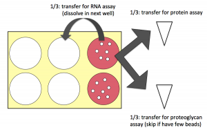 Bead preparation for three assays.
- About 1/3 of your beads will be used to measure protein content: move these to an eppendorf tube. The goal is about 10-15 (2-3 mm) beads per tube.
- For large beads (4-5 mm), you might use only 5-10 beads, and for very small beads (<1 mm), you might use 20 or more.
- Another 1/3 will be used to measure proteoglycan content; these whole beads can also be moved to an eppendorf tube.
- The final 1/3 will be used to isolate RNA. Using a sterile spatula, transfer the beads into a fresh well of your 6-well plate. This transfer step is to exclude any cells that are growing on the bottom of the plate (as opposed to actually in the beads) from analysis.

Samples for RNA Isolation
- Rinse the transferred bead-cell constructs with 4 mL of warm PBS, then aspirate the buffer.
- If your beads are very fragile, you might want to skip the PBS rinse, and directly proceed to step 2.
- Add 3 mL of pre-warmed EDTA-citrate buffer, and incubate at 37 °C for 10 min.
- Meanwhile, prepare the beads for the protein and proteoglycan assays as described below. All the materials that you need are in eppendorf tubes in the fridge.
- Now recover your cells:
- Add 3 mL of warm complete culture medium, pipet up and down to break up the beads (you may find this easier with a 1 mL pipetman rather than a serological pipet), and transfer to a 15 mL conical tube.
- Spin the cells down at 1900g for 6 min using the centrifuge that is in the TC room.
- Resuspend in ~ 1-1.5 mL of culture medium, and write down what you use. Mix thoroughly by pipetting, then set aside a 20 μL aliquot of your cells for counting, and put the rest of the cells into another eppendorf tube.
- If you have very few cells based on your Day 3 observations and/or having very few beads, you might consider skipping the cell count, and instead keeping all of the cells for RNA isolation. If you have too few cells to get a reliable cell count, you are not losing valuable information for your report in any case. And if you have so few cells that taking some of them for a count compromises your other data, then that outcome would not be preferable to missing the cell count.
- While one of you begins the spin in the main lab (see Part 2), the other should count your cell aliquot similarly to how you did on Day 2. This time, mix 10 μL of Trypan blue with your 20 μL of cells rather than using 90 μL, so we can conserve cells. Separately calculate the approximate numbers of live (yellowish) and of dead (blue) cells.
- Recall that you must multiply by 10,000 (and your dilution factor) to convert a hemacytometer cell count to a live cells/mL concentration.
Samples for Protein Extraction
- Per eppendorf tube (typically 10-15 beads), add 133 μL of cold EDTA-citrate buffer (not from the warm conical!), and pipet up and down for 20-30 seconds to dissolve the beads. Be thorough while limiting bubbles as best you can. The resulting solution may be viscous.
- Pipet 33 μL of 0.25 M acetic acid into each eppendorf tube.
- Finally, pipet 33 μL of 1 mg/mL pepsin (in 50 mM acetic acid) into each tube and mix well.
- Move your eppendorf tubes into the rack in the 4 °C fridge. Tomorrow the teaching faculty will move them to an elastase solution (also at 4 °C) to break down the polymeric collagen to more readily measured monomeric collagen.
Samples for Proteoglycan Extraction
- Soak your beads for a few minutes in pre-warmed PBS, and then remove as much of the PBS as possible. Shoot to have as little pink tint to the beads as possible, as it is known to interfere with the proteoglycan assay. Repeat the soak step a second time with fresh PBS, if it seems to help.
- Add 250 μL of papain solution to your beads. The papain is in an EDTA-citrate buffer base.
- When the first partner goes to the main lab, s/he should take this tube to the 60 °C heat block. After 24 hours, the samples will be moved to the freezer.
Part 2: RNA isolation and measurement
Because you are preparing RNA, you will have to take special precautions during this part. RNA is strikingly different from DNA in its stability. Consequently it is more difficult to work with RNA in the lab. It is not the techniques themselves that are difficult; indeed, many of the manipulations are nearly identical to those used for DNA. However, RNA is rapidly and easily degraded by RNases that exist everywhere. There are several rules for working with RNA. They will improve your chances of success. Please follow them all.
- Use warm water on a paper towel to wash lab equipment, such as microfuges, before you begin your experiment. Then wipe them down with “RNase-away” solution.
- Wear gloves when you are touching anything that will touch your RNA.
- Change your gloves often.
- Before you begin your experiment, clean and prepare your work area: (1) remove all clutter, (2) wipe down the benchtop with warm water and “RNase-away,” and (3) lay down a fresh piece of benchpaper and/or mark off the area with tape. This last step serves as a reminder to always wear your gloves when touching items in that area.
- Use RNA-dedicated solutions and if possible RNA-dedicated pipetmen.
- Get a new box of pipet tips from the RNA materials area and label their lid “RNase FREE” if the lid is not yet labeled.
- Pellet the cells for RNA isolation back in the main lab (8 min at 500 g).
- Remove the supernatant from your cell pellets using pipet tips from an RNase free tip box.
- Discard this and other supernatants in a conical waste tube. As you may remember from Module 1, the lysis reagent you will use shortly is not compatible with bleach.
- Now, in the fume hood, add 350 μL RLT with β-mercaptoethanol to each cell sample – vortex or pipet to mix.
- If you have more than 5 million cells, you will need to double the amount of RLT used - talk to the teaching faculty.
- Add each cell lysate to a separate QIAshredder column, which is used to remove particulate matter. Microfuge the columns (over a 2 mL collection tube) for 2 min at max speed. Save the flowthrough!!!
- Add 1 volume (slightly > 350 μL) of 70% ethanol to each lysate and pipet to mix.
- Apply each sample (including any precipitate) to a separate RNeasy mini column (over a tube). Microfuge for 15 sec and discard the flowthrough.
- Add 700 μL RW1 buffer to each column. Microfuge 15 sec and discard the eluant again.
- Add 500 μL RPE buffer atop the columns, microfuge as before (15 sec), and discard the flowthrough.
- Repeat the addition of 500 μL RPE, but this time centrifuge for 2 min. prior to discarding the flowthrough.
- Transfer the columns to fresh 2 mL collection tubes.
- Centrifuge the column/tube "dry" for 1 min. Running a column like this helps to fully dry it, and to prevent carryover of ethanol.
- Trim the caps off of two new 1.5 ml eppendorf tubes (save the caps!) and label the sides of the tubes.
- Transfer the dried columns into the trimmed eppendorf tubes and elute the RNA from the columns by adding 30 μL of RNase-free water to each. Microfuge for 1 min, then cap the tubes and store the eluants on ice.
- Measure the concentration of your RNA samples. First prepare dilutions: 15 μL of of each in 385 μL sterile water. (The water does not strictly speaking have to be RNase-free since the RNA can be degraded and still give legitimate readings in the spectrophotometer.)
- This time you will work in "wavelength scan" mode on the spectrophotometer, rather than take readings only at 260 and 280 nm, as you may learn something about your samples from the shape of the entire curve from 250-290 nm.
- Begin with the cuvette containing blanking solution, and hit Blank on the spectrophotometer.
- Proceed to take an absorbance scan of each RNA sample. Record the 260 nm and 280 nm absorbance values in your notebook. You can simply touch your finger to the onscreen spectrum for coarse wavelength selection, and then touch the onscreen arrows for fine selection.
- Note the RNA concentrations of your samples in the table below, using the fact that 40 μg/mL of RNA will give a reading of A260 = 1. Also calculate the 260:280 ratio, which should approach 2.0 for very pure RNA.
- Ideally, you will use 500 ng of RNA in each RT reaction. However, it's also useful to have all reactions to start with an equal amount of RNA template. (Although we will normalize with GAPDH transcripts, the more similar the samples are to begin with, the better.) At most you can use 7.5 μL of RNA per reaction. If you can use 500 ng per reaction within the above contraints, do so. Otherwise, figure out which one of your samples is limiting, and scale the other added sample amount so they are equal. If one sample is very low, or even below the detection limit of the spectrophotometer, don't scale to it and risk getting no data from either sample. Finally, note that if you use less than 7.5 μL RNA, water should be added to make up the difference. The table below may be helpful as you carry out your calculations.
| Sample | A260 | Measured RNA conc. (μg/mL) | RNA conc. of undiluted stock (μg/mL) | Max RNA per rxn (ng in 7.5 μL) | Volume RNA needed per rxn | Volume water needed per rxn |
|---|---|---|---|---|---|---|
| 1: | ||||||
| 2: |
Part 3: RT reactions
- Set up your reactions on a cold block as usual. You will prepare one reaction for each of your samples. Random hexamer primers will be used so that all (we hope) transcripts are amplified. This approach is more convenient than adding unique primers for each transcript of interest.
- From one of the shared stocks, pipet 22.5 μL of RT master mix into each of two well-labeled PCR tubes. The master mix contains water, buffer, dNTPS, primers, and reverse transcriptase.
- Now you can add 7.5 μL of the appropriate RNA (or RNA and water as needed) to each tube.
- The following thermal cycler program will be used: 20 min at 25 °C, 30 min at 42 °C (reverse transcription step), and then cooling. After the RT is completed, the teaching faculty will store the samples in the freezer until next time.
In whatever time remains today, you can continue work on your FNT or on the Module 3 mini-report. The steps to analyze your cell viability images are outlined below.
Part 4: Begin viability analysis (optional)
Starting today or as late as Day 6, you will use an image analysis program called ImageJ to quantify your live/dead data. This program is offered free of charge by the NIH (National Institutes of Health).
Cell Counting
Your goal for this section will be to compare the effort required for, and the resulting accuracy of, manually counting live and dead cells vs. doing so by semi-automated image analysis. After you are done, you might consider under what conditions you might prefer one method or the other.
If you don't have many cells to look at, extra data is available on today's Talk page.
- Open your live cell image (green filter) by selecting File → Open
- Choose the line tool, and draw a line across the diameter of a typical cell
- Select Analyze → Set Scale, and put 10 μm in under Known Distance
- note: in lieu of using the exact pixel information from the camera, we simply are putting in the average size of a cell
- Convert your image to grey scale using Image → Type → 8-bit
- Now you must somehow select your cells out from the background
- One way to do this is by choosing Process → Binary → Make Binary. However, you might find that clusters of cells are ‘read’ as a single cell.
- An improved method is to use Image → Adjust → Threshold. You can set the upper- and lower-bound intensities that define objects in your image. Play with the intensity sliders until your cells are mostly filled in with a red colour, but not overlapping with other cells whenever possible.
- Now you can count the objects. Choose Analyze → Analyze Particles, and select Show →Outlines, Display Results, Summarize, and Record Stats. Also choose a reasonable area (not diameter!) range for objects that are cell-sized.
- Try to play around with this process for a bit – are there any further changes you can make so the automated algorithm is as good as your eye?
- Record your final results (manual and best automated) in your notebook, for each sample that you have data for. Don’t forget to also manually count the dead cells, and subtract this number from the live cells (since the filter we used shows both green and red cells at once).
Statistical Analysis
Once you have cell counts (whether automated or manual) that you are happy with, you can do some basic statistical analysis. Isn't it nice to have way fewer samples than in Module 2?
- If you like, you may again download the linked Excel file as a framework to carry out the basic statistical manipulations below. The file is modified from one originally written by Professor Bevin Engelward.
- Find and plot 95% confidence intervals for the live cell counts and/or live cell percentage for each of your two samples.
- What are the advantages and disadvantages of looking at counts versus percentages? In what situations would looking at counts be misleading?
- Compare the means (count and/or percentage) of your two samples. At what confidence level (if any) are they different?
For next time
- Write a brief response (250 ± 50 words) to one of the excerpts that were handed out in lecture and lab.
- These excerpts are drawn (with some editing) from previous 20.109 student essays about the prospect of standardization in tissue engineering.
- You may revise the response you started during lecture, or write a brand new one.
- Due on M3D5 (one week from today).
- The primary assignment for this experimental module will be for you to develop a research proposal and present your idea to the class. For next time, please describe five recent findings that might define an interesting research question. You should hand in a 3-5 sentence description of each topic – in your own words – and cite an associated reference from the scientific literature. The topics you pick can be related to any aspect of the class, i.e. DNA, system, or cell/biomaterial engineering. During lab next time, you and your partner will review the topics and narrow your choices, identifying one or perhaps two topics for further research.
- Note: for now, you do not have to have a novel research idea sketched out; you simply have to describe five recent examples of existing work. However, you can start to brainstorm how to build off of those topics into something new if you want to get ahead of the game.
- Due on Tuesday, April 29th, in 16-220 between 11 AM and 12 PM. We will make this space available for the hour to partners who want to complete their initial research idea discussions (see description in M3D5 Protocols, Part 4) right away.
Reagent list
- Culture medium as on Day 1
- Release Buffer for Beads
- 150 mM NaCl
- 55 mM sodium citrate
- 30 mM EDTA
- For protein extraction
- 0.25 M acetic acid
- pepsin (Sigma), at 1 mg/mL in 50 mM acetic acid
- TBS buffer (pH 7.8-8.0), NaOH to get pH to 8.0, 1 mg/mL elastase in TBS
- 10X TBS is 1M Tris, 2M NaCl, 50 mM CaCl2
- For proteoglycan extraction
- 150 mM NaCl, 55 mM sodium citrate, 5 mM EDTA, 5 mM cysteine hydrochloride, 0.56 U/mL papin
- For RNA extraction
- Qiagen QIAshredder columns
- Qiagen RNeasy kit
- RLT needs to have βmercaptoethanol added before use (just an aliquot, stable for 1 month)
- buffer PE needs to have ethanol added prior to first use
- RT Master Mix
Materials are from Applied Biosystems unless otherwise noted. Concentrations are final.
| Component | Concentration |
|---|---|
| Random hexamer Primers | 1.25 μM |
| dNTPs (Promega) | 1 mM |
| RNase inhibitor | 0.5 U/μL |
| Multiscribe muLV (murine leukemia virus) reverse transcriptase | 1.25 U/μL |
| PCR buffer and MgCl2 | N/A, multi-component |
Next Day: Initiating transcript and protein assays
Previous Day: Testing cell viability