Understanding the lock-in amplifier
Lock-in signal detection
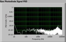
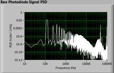
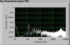
The plots below show typical power spectral density measurements of noise in the 20.309 lab — a mix of optical and electronic noise. Fluorescent lighting creates a very strong technical noise at 120 Hz and harmonics. The lock-in technique used in the DNA lab involves modulating the blue light that excites the fluorescent dye in the sample to move the signal spectrum from the riotous low frequency realm to a calmer range of frequencies. Lock-in signal detection provides some immunity to the very noisy lab environment.
Noise in lab the may look different than in previous semesters, so it may be useful to measure the noise spectrum before settling on a modulation frequency for your lock-in amplifier.
| |
||
| |
|
|
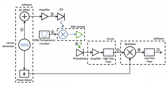
A block diagram of the lock-in scheme is shown below. Implementing lock-in detection requires the ability to modulate the LED output with a carrier frequency and requires signal processing (in software in our case) to recover the non-modulated signal. In your case the non-modulated signal is the fraction of dsDNA versus time. To support these functions, the LED circuit must be modified to include a feedback brightness controller. In addition, the photodiode amplifier must be modified to accommodate the change in signal frequency range. In the control software, you will need to choose the LED modulation frequency as well as all filter frequencies to support your design.
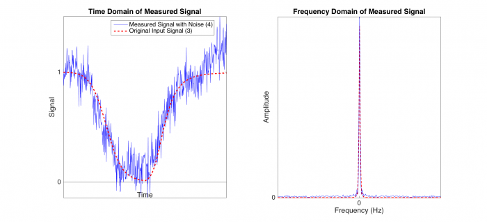
Figure 1. Point 3 on the above block diagram represents our original input signal (red dashed line), in which dsDNA at room temperature is heated and is cooled. However, as we have seen in Part 1 of the DNA Melting lab, the signal we retrieve contains some amount of noise (blue line). In this simulation, we have modeled room noise with a Brown noise generator in Matlab because Brown noise is stronger in low frequencies, similar to the room noise. In the frequency domain plot (on right), the original input signal (red) contains low frequency.
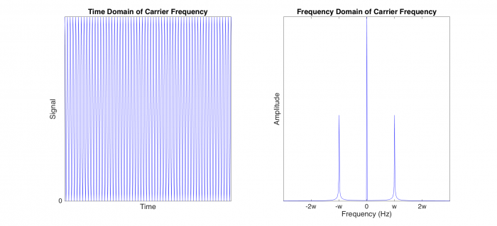
Figure 2. To implement lock-in detection, we must first modulate the LED output so that it flashes at the carrier frequency w. The brightness of the LED depends on how much current it draws; however, we cannot feed the LED negative current because the LED is directional. Our carrier frequency, cos(wt), must have an offset added to the signal so that all voltage values are above zero, as shown in the left plot, which corresponds to point 2 in the block diagram. In the right plot, we have peaks at w and -w, as well as at 0 because of the added offset.
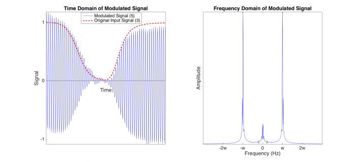
Figure 3. When the blue LED flashes at the carrier frequency, the light excites the fluorescent DNA sample. In the right plot, representing point 5 in the block diagram, the blue line shows the output of the amplifier after current is collected from the photodiode. The modulated signal has the frequency of the carrier frequency w, but the amplitude is approximately that of the original input signal (dashed red line). Deviations from the original input can be attributed to the photonic noise that is also collected by the photodiode.
Because noise is not time varying, after modulation, the noise still stays at low frequencies. The peaks about 0 Hz in the right plot represent noise. In contrast, the original input signal has now been modulated to the carrier frequency w, and so the modulated signal is represented in the peaks in the right plot at w and -w.
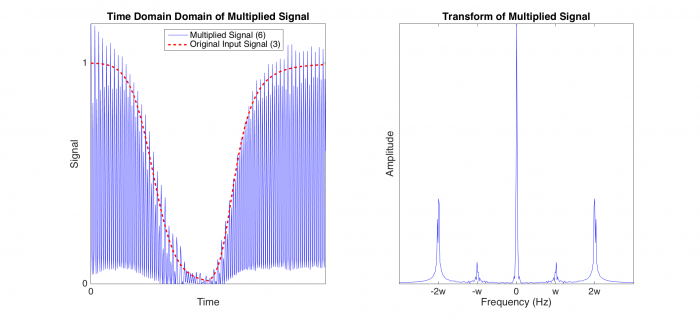
Figure 4. The next step in lock-in detection is to multiply the signal obtained at point 5 in the block diagram and multiply it by the carrier frequency again (but without the offset). The resulting signal, which corresponds to point 6 on the diagram, now appears to be at twice the frequency than in the previous figure.
If we look at the plot on the right, we see how the transform is the result of multiplying the transform in Figure 3 by the transform of Figure 2. If we take the transform of Figure 3 and center it about both w and -w, we will move our signal to -2w and 0 Hz on one side and 0 and 2w Hz on the other side. The noise, which was originally at 0 is now shifted to -w on one side and w on the other side. Because the original input signal is present at 0 Hz, we can use a low-pass filter to retrieve the signal without the noise if we choose a filter cutoff frequency of less than w/2.
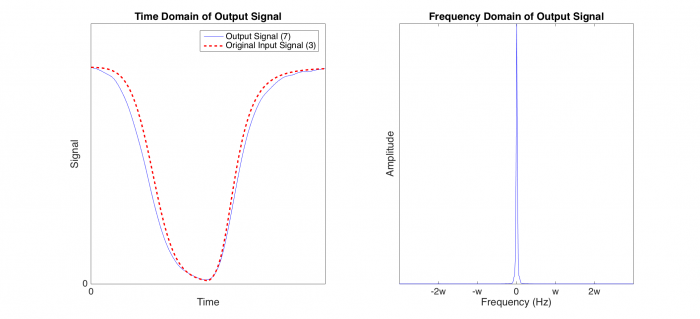
Figure 5. In our MATLAB simulation, we generated a low-pass filter and passed the signal from Point 6 through it. The output signal at point 7 (blue line) is our lock-in amplifier's approximation of the input signal combined with the noise gained from experimentation. The output signal is very close to the original input signal (dashed red line), and can be made to be an even better approximation by using a higher resolution low-pass filter or choosing a different carrier frequency.
MATLAB Simulation
The following Matlab code was used to generate the figures above.
close all
clear all
clc

% Simulation of different steps in the lock-in amplifier
%
% Requires DnaFraction.m as a function, as documented in DNA Melting:
% Simulating DNA Melting - Basics wiki page. Steps correspond with block
% diagram shown in Understanding the Lock-in Amplifier wiki page.
%
% First, we generate a signal for DNA melting by specifying ideal
% conditions, creating a time vector, and modeling temperature.

simulationLength = 300;                               % 5 min sim for each melting and cooling
sampleRate = 1;                                       % 1 Hz sample rate
sim1 = struct();                                      % create empty struct for sim results
sim1.concentration = 1E-6;                            % 1 micromolar concentration
sim1.deltaS = -184;                                   % cal / (mole-K)
sim1.deltaH = -71E3;                                  % cal / mole
sim1.initialTemperature = 293;                        % approx. room temperature
sim1.finalTemperature = 363;                          % 363 K = 90 C
sim1.time = 0:(1./sampleRate):(simulationLength);       % create time vector (units: seconds)
sim1.coolingConstant = 200;
% use exp function to model heating and cooling
sim1.temperature = ...                                           % Melting
    (sim1.initialTemperature - sim1.finalTemperature) .*   ...   % T_i - T_f *
    exp(-sim1.time ./ sim1.coolingConstant) +   ...              % e^(-t/tau) +
    sim1.finalTemperature;                                       % T_f
sim2 = struct();
sim2.initialTemperature = sim1.temperature(end);
sim2.finalTemperature = sim1.initialTemperature;                 % Cooling
sim2.time = (simulationLength+sampleRate):(1./sampleRate):(2*simulationLength+sampleRate);
sim2.temperature = ...
    (sim2.initialTemperature - sim2.finalTemperature) .*   ...   % T_i - T_f *
    exp(-sim1.time ./ sim1.coolingConstant) +   ...              % e^(-t/tau) +
    sim2.finalTemperature;                                       % T_f
sim1.time = [sim1.time,sim2.time];
sim1.temperature = [sim1.temperature,sim2.temperature];

% Signal based on simulation
dnaFractionMelting = DnaFraction(sim1.concentration, sim1.temperature,...
    sim1.deltaS, sim1.deltaH);

% Model room noise using MATLAB function to generate Brown noise.
% The 'Understanding the lock-in amplifier' wiki page shows examples of
% actual noise in the room.

coloredNoiseGenerator = dsp.ColoredNoise(2,length(dnaFractionMelting),1);
brownNoise = step(coloredNoiseGenerator);
brownNoiseNorm = (brownNoise-min(brownNoise))/(max(brownNoise)-min(brownNoise))-0.4;

% First figure demonstrates that because signal and noise occupy the same
% frequencies, a bandpass filter cannot be used to remove noise from
% signal. Brown noise is added to signal and white gaussian noise is added
% on top of that.

dnaFractionNoise = awgn((dnaFractionMelting + 0.5*transpose(brownNoiseNorm)),20);

brownNoiseTransform = abs(fftshift(fft(brownNoiseNorm)));
noiseFreqs = linspace(-sampleRate/2, sampleRate/2, length(brownNoiseTransform));
signalTransform = abs(fftshift(fft(dnaFractionMelting)));
signalFreqs = linspace(-sampleRate/2, sampleRate/2, length(signalTransform));
signalNoiseTransform = abs(fftshift(fft(dnaFractionNoise)));
signalNoiseFreqs = linspace(-sampleRate/2, sampleRate/2, length(signalNoiseTransform));

figure(1)
subplot(1,2,1)
plot(sim1.time, dnaFractionNoise, 'Color', 'blue')
xlabel('Time','FontSize', 14)
ylabel('Signal','FontSize', 14)
title('Time Domain of Measured Signal','FontSize', 18)
ax = gca;
ax.XAxisLocation = 'origin';
axis([0 600 -inf inf])
set(gca,'xtick',[0],'ytick',[0,1],'FontSize', 14)
hold on
plot(sim1.time, dnaFractionMelting, '--', 'LineWidth', 2,'Color','red')
hold off
l=legend('Measured Signal with Noise (4)','Original Input Signal (3)');
set(l,'FontSize',13);

subplot(1,2,2)
plot(signalFreqs, signalTransform,'--', 'LineWidth', 1.5,'Color','red')
hold on
plot(signalNoiseFreqs, signalNoiseTransform,'Color', 'blue')
title('Frequency Domain of Measured Signal','FontSize', 18)
axis([-0.2 .2 0 inf])
xlabel('Frequency (Hz)','FontSize', 14)
ylabel('Amplitude','FontSize', 14)
set(gca,'xtick',[0],'ytick',[0],'FontSize', 14)
hold off

% Second figure shows the carrier frequency. This is the frequency (w) that we
% will move the signal to separate it from the noise. The carrier frequency
% is offset in order to prevent giving negative values to the LED.

carrierFreq =cos(2*pi*0.1*sim1.time);
carrierFreqOffset = carrierFreq + 1;       % DC Offset

figure(2)
subplot(1,2,1)
plot(sim1.time,carrierFreqOffset,'Color','blue')
title('Time Domain of Carrier Frequency','FontSize', 18)
xlabel('Time','FontSize', 14)
ylabel('Signal','FontSize', 14)
ax.XAxisLocation = 'origin';
set(gca,'xtick',[],'ytick',[0],'FontSize', 14)
axis([0 600 -inf inf])

carrierTransform = abs(fftshift(fft(carrierFreqOffset)));
freqSpaceCarrier = linspace(-sampleRate/2, sampleRate/2, length(carrierTransform));

subplot(1,2,2)
plot(freqSpaceCarrier,carrierTransform, 'Color','blue')
title('Frequency Domain of Carrier Frequency','FontSize', 14)
xlabel('Frequency (Hz)','FontSize', 14)
ylabel('Amplitude','FontSize', 14)
set(gca,'xtick',[-0.2,-0.1, 0, 0.1, 0.2],'xticklabel',{'-2w','-w','0','w','2w'},'ytick',[]...
    ,'FontSize', 14)
axis([-0.3 .3 1E-1 inf])

% The third figure demonstrates what happens when we modulate the the
% signal to the carrier frequency by multiplying the two. The noise is
% not time varying, so the amplitude spectrum of noise will remain about
% zero, while the signal will be moved to the carrier frequency.

modulatedSignal = (carrierFreq).*dnaFractionMelting;
modulatedSigNoise = modulatedSignal + 0.3*transpose(brownNoiseNorm);

figure(3)
subplot(1,2,1)
plot(sim1.time, modulatedSigNoise, 'b' )
title('Time Domain of Modulated Signal','FontSize', 18)
xlabel('Time','FontSize', 14)
ylabel('Signal','FontSize', 14)
ax = gca;
ax.XAxisLocation = 'origin';
set(gca,'xtick',[0],'ytick',[-1,0,1],'FontSize', 14)
axis([0 600 -inf inf])
hold on
plot(sim1.time, dnaFractionMelting,'--', 'LineWidth', 2,'Color','red' )
hold off
l=legend('Modulated Signal (5)','Original Input Signal (3)');
set(l,'FontSize',13);

modulatedSigNoiseFFT = abs(fftshift(fft(modulatedSigNoise)));
modFreq = linspace(-sampleRate/2, sampleRate/2, length(modulatedSigNoiseFFT));

subplot(1,2,2)
plot(modFreq,modulatedSigNoiseFFT,'b')
title('Frequency Domain of Modulated Signal','FontSize', 18)
xlabel('Frequency (Hz)','FontSize', 14)
ylabel('Amplitude','FontSize', 14)
axis([-0.3 .3 0 inf])
set(gca,'xtick',[-0.2,-0.1, 0, 0.1, 0.2],'xticklabel',{'-2w','-w','0','w','2w'},'ytick',[]...
    ,'FontSize', 14)

% The fourth figure demonstrates what happens when you multiply the
% modulated signal by the reference frequency, which is at the same
% frequency as the original carrier frequency. The signal has now moved
% back to the origin, and the noise is moved to the carrier frequency.

figure(4)
subplot(1,2,1)
multipliedSignal = modulatedSigNoise .* carrierFreq;
plot(sim1.time, multipliedSignal,'b')
title('Time Domain Domain of Multiplied Signal','FontSize', 18)
xlabel('Time','FontSize', 14)
ylabel('Signal','FontSize', 14)
set(gca,'xtick',[0],'ytick',[0,1],'FontSize', 14)
axis([0 inf 0 inf])
hold on
plot(sim1.time, dnaFractionMelting,'--', 'Color','red', 'LineWidth', 2)
hold off
l=legend('Multiplied Signal (6)', 'Original Input Signal (3)');
set(l,'FontSize',13);

multipliedSigFFT = abs(fftshift(fft(multipliedSignal)));
multFreq = linspace(-sampleRate/2, sampleRate/2, length(multipliedSigFFT));

subplot(1,2,2)
plot(multFreq,multipliedSigFFT,'b')
title('Transform of Multiplied Signal','FontSize', 14)
xlabel('Frequency (Hz)','FontSize', 14)
ylabel('Amplitude','FontSize', 14)
axis([-0.3 .3 0 inf])
set(gca,'xtick',[-0.2,-0.1, 0, 0.1, 0.2],'xticklabel',{'-2w','-w','0','w','2w'},'ytick',[]...
    ,'FontSize', 14)

% Lowpass filter to retrieve original signal

lowpassfilter =fir1(60, 0.02/0.5);
y = conv( multipliedSignal, lowpassfilter,'valid');
t2 = linspace(0,2*simulationLength+sampleRate,length(y));

figure(5)
subplot(1,2,1)
plot(t2,y,'b')
title('Time Domain of Output Signal','FontSize', 18)
xlabel('Time','FontSize', 14)
ylabel('Signal','FontSize', 14)
set(gca,'xtick',[0],'ytick',[0,1],'FontSize', 14)
axis([0 inf 0 0.6])
hold on
plot(sim1.time,0.5*dnaFractionMelting,'--','Color','r', 'LineWidth',2)
hold off
l=legend('Output Signal (7)', 'Original Input Signal (3)');
set(l,'FontSize',13);

outputFFT = abs(fftshift(fft(y)));
outputFreq = linspace(-sampleRate/2, sampleRate/2, length(outputFFT));

subplot(1,2,2)
plot(outputFreq,outputFFT,'b')
title('Frequency Domain of Output Signal','FontSize', 18)
xlabel('Frequency (Hz)','FontSize', 14)
ylabel('Amplitude','FontSize', 14)
axis([-0.3 .3 0 inf])
set(gca,'xtick',[-0.2,-0.1, 0, 0.1, 0.2],'xticklabel',{'-2w','-w','0','w','2w'},'ytick',[]...
    ,'FontSize', 14)
References

