Optical Microscopy Part 3: Resolution and Stability
Overview
Congratulations on completing part 2. You made a functioning epifluorescence microscope. How cool is that?
In this part of the lab, you will measure the resolution of your microscope using tiny, fluorescent microspheres as sources. Next, you will quantify the stability of your microscope by tracking immobile beads. In part 4 of this lab, you will characterize the diffusive motion of particles in different rheological environments by tracking fluorescent microspheres. Your microscope will act as a position detector. To prepare for these measurements, you will measure the position noise of your instrument to establish a baseline performance parameter.
Instructions
Measuring resolution
One of the most commonly used definitions of resolution is the distance between two point sources in the sample plane such that the peak of one source’s image falls on the first minimum of the other source’s image. This suggests a procedure for measuring resolution: image a point source; measure the peak-to-trough distance; and divide by the magnification. In this part of the lab, you will use this method to estimate the resolution of your microscope.
A practical problem with this method is that true point sources are difficult to come by. If you are using a telescope, stars are readily available approximate point sources. In microscopy, people usually use tiny, fluorescent beads with diameters of 100-190 nm. These beads are small enough to be considered point sources. You will use nonlinear regression to estimate the resolution of your microscope from an image of the tiny beads. Unfortunately, beads small enough for this purpose are not very bright. Imaging them can be challenging. Your microscope must be aligned very well to get good results.
You will use image processing functions to locate the beads in your image and fit a Gaussian function to them. Gaussians are more amenable to nonlinear regression than Bessel functions, and they are a very good approximation. It is straightforward to convert the Gaussian parameters to Rayleigh resolution. See Converting Gaussian fit to Rayleigh resolution for a discussion of the conversion.
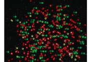
- Make an image of a sample of 170 nm fluorescent beads with the 40X objective. (Several dozens to hundreds of PSF spheres should be captured in your image.)
- Use 12-bit mode on the camera and make sure to save the image in a format that preserves all 12 bits.
- Use
imhistto ensure that the image is exposed properly.- Since there are a very small number of bright pixels, plot the histogram counts on a logarithmic scale.
- Include the image and the histogram in your lab report.
- Use image processing functions to locate non-overlapping, single beads in the image.
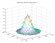
- Use nonlinear regression to fit a Gaussian to each bead image.
- Convert the Gaussian parameters to resolution.
- Report the results in your lab report.
- This page has example MATLAB code.
- Discuss how the measured resolution compares with the theoretical value.
Stability of microscope for particle tracking
The accuracy of optical particle tracking may be limited by mechanical and optical phenomena. Vibration and drift are a source of additive noise. Shot noise and CCD readout noise in the image of a particle bring about uncertainty in the estimate of its centroid. Excessive vibration can frequently be corrected by improving the mechanical support structure of the instrument. Most stages can be locked to reduce drift. Shot noise is fundamental; however, its relative contribution to the total signal can be minimized by ensuring that the optical system is functioning at peak efficiency.
Before attempting to make measurements with particle tracking (Part 4), it is essential to determine the performance characteristics of the instrument to be used. This can be accomplished by measuring a specimen with known characteristics. Perhaps the most foolproof choice is a sample with fixed particles. Any measured variation in the fixed sample is noise.
In order to analyze your data, you will need to write code in Matlab. It is helpful to make sure your code is working before you collect data (especially for Part 4). You may download this set of Matlab files to help you get started: File:Matlab Code Following Things 2.zip. Please note that you should take any code you download from the internet (including ones from this class) with a grain of salt--you will want to verify your code is working the way it should and that any bugs are fixed. One way to help test your code is to use it on simulated data, where you know what the output should be. You will find this exercise useful.
- To verify that your system is sufficiently stable for accurate particle tracking, monitor a dry specimen containing 0.84μm fluorescent beads.
- Bring a slide with fixed beads into focus. Choose a field of view in which you can see at least 3 beads with the 40× objective. Limit the field of view to only those beads by choosing a region of interest (ROI) with the UsefulImageAcquisition tool.
- Track the beads for 3 minutes in a Matlab video and save the centroids with a frame rate of your choice and make a note of it.
- Use the Matlab function
track(be sure to limit the algorithm to a small region of interest around the beads, otherwise Matlab will struggle!) to separate the centroids into individual trajectories, $ \vec r_n(t) $, where $ t = nT $ and $ T $ is the inverse of the frame rate you set above. - Compute the difference of the trajectories for two particles, $ \vec r_-(t) = {{\vec r_1(t) - \vec r_2(t)} \over \sqrt{2}} $. (Why is the square root of 2 necessary?)
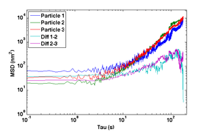
- Compute and plot the mean squared displacement (MSD) of $ r_- $ as a function of time interval and compare to the MSD of the actual particle tracks, $ \left \langle {\left | \vec r(t+\tau)-\vec r(t) \right \vert}^2 \right \rangle $ for intervals $ \tau=nT $ up to 180 s.
- Why does the MSD of the particle trajectory increase while the difference trajectory stays about constant over the range of lag times τ?
- Can you take advantage of this property to decrease the error in measurements of unknown samples?
- Make any necessary adjustments to your microscope and repeat this particle-tracking procedure to attain sufficient stability:
- The MSD from the difference trajectory should start out less than 100 nm2 at t = 1 s and still be less than 1000 nm2 for t = 180 s.
Report
Find and follow all guidelines on the Microscopy report outline wiki page.
- Resolution
- Procedure
- Document the samples you used and how you captured images (camera settings, software used, etc…)
- Data
- Include an image of the PSF sample indicating which beads were used for resolution measurement..
- Analysis and Results
- Report the resolution you measured. Make sure to include N and a measure of uncertainty.
- Show sample Gaussian fits.
- Explain the Matlab algorithm used for data analysis.
- Discussion
- Compare the measured value to the theoretical value.
- Include a thorough discussion of error sources. Do not comment on insignificant sources of error. To determine which error sources are significant, and which are not, you must think carefully about the uncertainty related to each error source and estimate its magnitude and sign. Include these estimates in your report along with your estimate of the combined, total uncertainty. It may be helpful to list out the error sources in a table, including a category for the error source, type of error (random, systematic, fundamental, technical, etc.), the magnitude of the error, and a description and way to minimize each one.
- Procedure
- Stability
- Procedure
- Document the samples you used and how you captured images (camera settings, frame rate, total number of frames, exposure, software used, etc…)
- Data
- Show an example frame from the stability movie.
- Plot two or more example bead trajectories for each of the samples. (Hint: If you subtract the initial position from each trajectory, then you can plot multiple trajectories on a single set of axes.)
- Analysis and Results
- Plot MSD versus time interval τ for individual and difference tracks using log-log axes.
- Provide a bullet point outline of data analysis methodology.
- Discussion
- What are the benefits and drawbacks of differential tracking?
- Include a thorough discussion of error sources.
- Procedure
Optical microscopy lab
Code examples and simulations
- Converting Gaussian fit to Rayleigh resolution
- MATLAB: Estimating resolution from a PSF slide image
- Matlab: Scalebars
- Calculating MSD and Diffusion Coefficients
Background reading
- Geometrical optics and ray tracing
- Physical optics and resolution
- Optical aberrations
- Aperture and field stops
- Optical detectors, noise, and the limit of detection
- Manta G032 camera measurements
- Understanding log plots
References


