20.109(S12):Assess protein function (Day7)

Introduction

This is it, folks! Moment of truth. Time to find out how the proteins that you worked so hard to make and purify really behave.

Today you will obtain titration curves against calcium for your wild-type and mutant proteins using an automated fluorescence plate reader. This machine reads multiple samples in a standard format – in our case, a 96-well microtiter plate. The output is a grid of up to 96 fluorescence values, for rows A-G and columns 1-12, which is amenable to analysis with a program like Excel.

In order to further benefit from this high-throughput testing format, you will make friends with the multichannel pipet, a purely mechanical rather than digital aid for repetitive experiments. This tool allows you to suck up and expel equivalent volumes of multiple identical samples (usually 8-12 at a time) with just one stroke. You will use this type of pipet to fill each row of a microtiter plate with one type of protein sample, and each column with a different concentration of calcium. Although a multichannel pipet can be sufficient for a typical research lab, in pharmaceutical companies that may be assaying thousands of samples a day, yet more steps of automation and scaling up are required, such as robotic pipet arms that obviate the need for manual pipetting at all. The degree of automation commercially available, or developed ‘in-house’ in a certain lab or corporation, depends in part on the frequency with which a certain assay is used. Assays used by many different labs and companies (such as fluorescence or absorbance spectrophotometry) are likely to breed commercially available high-throughput machines.

Signal:noise in arbitrary data collection. Background measurements (open circles), sample measurements (closed circles), and average values (short horizontal lines) are shown. The short line without any data points represents the reduction in average signal when background is subtracted. All measurements are with respect to an arbitrary vertical axis; the long horizontal line represents a measurement of zero.

While the concept of scale is a pragmatic concern, a perhaps more substantive topic of interest to us today is that of confidence in our results. As you are probably well-aware, every manipulation and measurement you make in the lab has an error associated with it. For example, consider the ubiquitous P200 pipetman. According to one pipet manufacturer, its accuracy is 1% (slightly worse at the lowest volumes). So an attempt to pipet 100 μL would result in an actual volume of 99-101 μL from the error of the instrument alone, which could be further compounded by a sleepy pipet operator, say. The precision of a pipet is typically better than its accuracy, 0.25% for the example given above. Precision refers to the reproducibility of a given measurement, not its absolute accuracy. This simple example demonstrates the general principles applicable to other types of error.

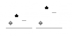
You will attempt to get a sense of the overall error of today’s experiment by running your protein samples in duplicate. That is, for each protein-calcium combination, you will perform two independent measurements. These measurements can then be averaged to smooth out your data, and hopefully improve the signal to noise ratio - where signal here refers to true differences between samples mixed with different amounts of calcium, and noise means inherent fluctuations in the system due to error. Noise in this experiment can also refer to background fluorescence of the sample buffer. Thus, another way to maintain a reasonable signal:noise ratio is by keeping our protein fairly concentrated, so that the absolute fluorescence values we obtain are high compared to the background. The figure at right demonstrates the above concepts. Scatter in the data (not all of the circles are at the same height) is one kind of noise. The level of background is another kind of noise: the left-hand data has a relatively low signal and thus poor signal:noise ratio, while the right-hand data has a relatively high absolute signal and improved signal:noise ratio.

Beginning today or at a later time before your reports are due (such as next week's office hours), you will analyze the raw data obtained today. Although you should be able to produce reasonable titration curves by following the example of Nagai, the introduction/review of binding constants below may help contextualize your analysis.

Let’s start by considering the simple case of a receptor-ligand pair that are exclusive to each other, and in which the receptor is monovalent. The ligand (L) and receptor (R) form a complex (C), which reaction can be written

$ R + L \rightleftharpoons\ ^{k_f}_{k_r} C $

At equilibrium, the rates of the forward reaction (rate constant = $ k_f $) and reverse reaction (rate constant = $ k_r $) must be equivalent. Solving this equivalence yields an equilibrium dissociation constant $ K_D $, which may be defined either as $ k_r/k_f $, or as $ [R][L]/[C] $, where brackets indicate the molar concentration of a species. Meanwhile, the fraction of receptors that are bound to ligand at equilibrium, often called y or θ, is $ C/R_{TOT} $, where $ R_{TOT} $ indicates total (both bound and unbound) receptors. Note that the position of the equilibrium (i.e., y) depends on the starting concentrations of the reactants; however, $ K_D $ is always the same value. The total number of receptors $ R_{TOT} $= [C] (ligand-bound receptors) + [R] (unbound receptors). Thus,

$ \qquad y = {[C] \over R_{TOT}} \qquad = \qquad {[C] \over [C] + [R]} \qquad = \qquad {[L] \over [L] + [K_D]} \qquad $

where the right-hand equation was derived by algebraic substitution. If the ligand concentration is in excess of that of the receptor, [L] may be approximated as a constant, L, for any given equilibrium. Let’s explore the implications of this result:

• What happens when L << $ K_D $?

→Then y ~ $ L/K_D $, and the binding fraction increases in a first-order fashion, directly proportional to L.

• What happens when L >> $ K_D $?

→In this case y ~1, so the binding fraction becomes approximately constant, and the receptors are saturated.

• What happens when L = $ K_D $?

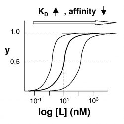
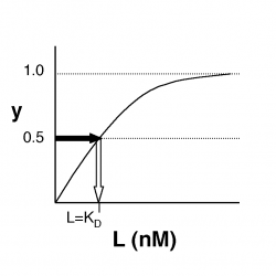
→Then y = 0.5, and the fraction of receptors that are bound to ligand is 50%. This is why you can read $ K_D $ directly off of the plots in Nagai’s paper (compare Figure 3 and Table 1). When y = 0.5, the concentration of free calcium (our [L]) is equal to $ K_D $. This is a great rule of thumb to know.

The figures at below demonstrate how to read $ K_D $ from binding curves. You will find semilog plots right particularly useful today, but the linear plot (left) can be a helpful visualization as well. Keep in mind that every L value is associated with a particular equilbrium value of y, while the curve as a whole gives information on the global equilibrium constant $ K_D $.

Simple Binding Curve The binding fraction y at first increases linearly as the starting ligand concentration is increased, then asymptotically approaches full saturation (y=1). The dissociation constant $ K_D $ is equal to the ligand concentration [L] for which y = 1/2.

Semilog Binding Curves By converting ligand concentrations to logspace, the dissociation constants are readily determined from the sigmoidal curves' inflection points. The three curves each represent different ligand species. The middle curve has a $ K_D $ close to 10 nM, while the right-hand curve has a higher $ K_D $ and therefore lower affinity between ligand and receptor (vice-versa for the left-hand curve).

Of course, inverse pericam has multiple binding sites, and thus IPC-calcium binding is actually more complicated than in the example above. The $ K_D $ reported by Nagai is called an ‘apparent $ K_D $’ because it reflects the overall avidity of multiple calcium binding sites, not their individual affinities for calcium. Normally, calmodulin has a low affinity (N-terminus) and a high affinity (C-terminus) pair of calcium binding sites. However, the E104Q mutant, which is the version of CaM used in inverse pericam, displays low-affinity binding at both termini. Moreover, the Hill coefficient, which quantifies cooperativity of binding in the case of multiple sites, is reported to be 1.0 for inverse pericam. This indicates that inverse pericam behaves as if it were binding only a single calcium ion per molecule. Thus, wild-type IPC is well-described by a single apparent $ K_D $.

When you write your research article, be sure to consider how changes in both binding affinity and cooperativity can affect the practical utility of a sensor.

Protocols

Two groups will begin with Parts 2 to 3, while everyone else begins with Part 1. The questions in Part 4 do not need to be handed in with your notebook, but are simply meant to guide your data analysis when you get to that stage. Your questions about Part 4 will be addressed during office hours.

Analysis must be completed and posted on today's Talk page by Friday at 5 pm (ideally much sooner!), so people can compare their own mutants to those of other teams doing similar work.

Part 1: SDS-PAGE

1. Last time you prepared cell-normalized -IPTG and +IPTG samples and added Laemmli sample buffer (containing SDS, etc.) to them. Now you will complete protein denaturing in preparation for PAGE, alongside a MW ladder.
   • The ladder is pre-stained and will be used to track gel progress. Unstained ladders contain a known amount of protein per band and can be used to estimate gross protein contents. We will not use one today, but they are a useful tool to be aware of.
2. Boil all 7 eppendorfs (including 15 μL of ladder!) for 5 minutes in the water bath that is in the fume hood.
3. You will be shown by the teaching faculty how to load your samples into the gel. You should load your samples according to the table below. Two groups will share each gel.
4. Note the starting and stopping time of electrophoresis, which will be initiated by the teaching faculty at 200 V, and run for 30-45 minutes.
5. Pry apart the plates using a spatula, and carefully transfer your gel to a staining box.
6. Add enough distilled water to cover the gel (say, 200 mL) and rinse the gel for 5 min on the shaker in the hood.
7. Repeat the rinse two more times with fresh water (~200 mL and 5 min incubation each time).
8. Add ~ 50 mL of BioSafe Coomassie, and incubate for at least 1 hour.
9. Empty the staining solution into the waste container in the fume hood - careful not to lose your gel!
10. Add 200 mL of water to your stained gel. Replace with fresh water just before leaving the lab if you have a chance.
11. Tomorrow, the teaching staff will transfer each gel to fresh water, then photograph them and post the results to the Day 6 Talk page.

Loading order and volumes

Loading volume is 10 μL for the ladder and 15 μL for your samples. Nothing goes in lane 1!

You may load your samples as -, -, -, +, +, + OR -, +, -, +, - +.
Either way, please use the order WT, E67K/T79P/M124S, X#Z.

Sample/Lane #	Sample Name	Sample/Lane #	Sample Name
2	Group 1	9	Group 2
3	Group 1	10	Group 2
4	Group 1	11	Group 2
5	Group 1	12	Group 2
6	Group 1	13	Group 2
7	Group 1	14	Group 2
8	Group 1, ladder	15	Group 2, ladder

Part 2: Prepare samples for titration curve

Tips for Success

Take great care today to limit the introduction of bubbles in your samples. When expelling fluid, pipet slowly while touching the pipet tip against the bottom or side of the well.

When using the multichannel pipet, always check to make sure all tips are getting filled - sometimes one tip may not be on all the way, and will pull up less volume than the others. If this happens, release the fluid, adjust the tip, and try again.

Protocol

Titration sample preparation

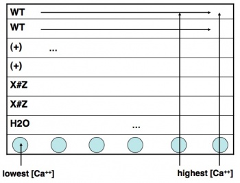
1. Take a black 96-well plate, and familiarize yourself with the scheme at right: top two rows are wild-type, next two rows are one of the E67K/T79P/M124S mutants, and the final two are your own mutant.
   • The dark sides of the plate reduce "cross-talk" (i.e., light leakage) between samples in adjacent wells, another potential contribution to error.
2. Transfer an aliquot of wild-type protein to a plastic reservoir. Use the multichannel pipet to add 30 μL of protein (per well) to the top two rows of your plate.
3. Take a fresh reservoir or use the next compartment in a divided reservoir, and repeat step 2 for your mutant proteins, adding each one to the appropriately labeled rows.
4. Finally, add plain water with only BSA (no IPC) to the seventh row of the plate, using the shared dedicated reservoir. (Why do you think we are including this row of solutions?)
5. Using shared reservoir #1 (lowest calcium concentration), add 30 μL to the top seven rows in the first column of the plate. Discard the pipet tips.
6. Now work your way from reservoirs #2 to #12 (highest calcium concentration), and from the left-hand to the right-hand columns on your plate. Be sure to use fresh pipet tips each time! If you do contaminate a solution, let the teaching faculty know so they can put out some fresh solution. Honesty about a mistake is far preferred here to affected every downstream experiment.
7. Finally, cover the plate with parafilm and wrap it in aluminum foil.

Part 3: Fluorescence assay

1. BPEC (the Biological Process Engineering Center) has graciously agreed to let us use their plate reader. Walk over to the BPEC instrument room with a member of the teaching staff.
2. You will be shown how to set the excitation (485 nm) and emission (515 nm) wavelength on the plate reader to assay your protein.
3. Your raw data will be posted on today's Talk page; alternatively, you can bring your own flash drive to recover the data immediately.

Part 4: Analysis

Begin by applying the practice analysis from Day 3, Part 5 of this module to your real data. Recall that here you plot titration curves in Excel and make a first crude estimate of K_D values. Next, you will use MATLAB to get improved estimates of K_Ds and also assess cooperativity. The MATLAB code is now up to date.

Preparation

1. Download these three files: S12_Fit_Main, Fit_SingleKD, and Fit_KDn. If using a computer in 16-336, the files will be available in the Downloads folder under your username. Move them to the username/Documents/MATLAB folder on your PC.
2. Double-click on the MATLAB icon to start up this software.
3. The main window that opens is called the command window: here is where you run programs (or directly input commands) and view outputs. You can also see and access the command history, workspace, and current directory windows, but you likely won’t need to today.
4. In the command window, type more on; this command allows you to scroll through multi-page output (using the spacebar), such as help files.
5. In addition to the command area, MATLAB comes with an editor. Click File → Open and select the program S12_Fit_Main. It has the .m extension and thus is executable by MATLAB. Read the introductory comments (the beginning of a comment is indicated by a % sign), and then input your fluorescence data.
6. Read through the program, and as you encounter unfamiliar terms, return to the workspace and type help functioname. Feel free to ask questions of the teaching faculty as well.
   • You might read about such built-in functions as logspace and nlinfit.
   • You will also want to open and read Fit_SingleKD – a user-defined function called by S12_Fit_Main – in the MATLAB editor.
   • If you type help function you will learn the syntax for a function header.
   • Note that a dot preceeding an operator (such as A ./ B or A .* B) is a way of telling MATLAB to perform element-by-element rather than matrix algebra.
   • Also note that when a line of code is not followed by a semi-colon, the value(s) resulting from the operation will be displayed in the command window.

Analysis

1. Once you more-or-less follow Part 1 of the program, type S12_Fit_Main in the workspace, hit return to run the program, and consider the following questions:
   • Why must the fluorescence data be transformed (from S to Y) prior to use in the model?
   • What $ K_D $ values are output in the command window, and how do they compare to the values you estimated from your Excel plots?
   • Figure 1 should display your wild type and mutant data points and model curves. How do they look in comparison to the curves you plotted in Excel?
   • Figure 2 should display the residuals (difference between data and model) for your three proteins. If the absolute values are low, this indicates good agreement between the model and the data numerically. Whether or not this is the case, another thing to look for is whether the residuals are evenly and randomly distributed about the zero-line. If there is a pattern to the errors, likely there is a systematic difference between the data and the model, and thus the model does not reflect the actual binding process well. What are the residuals like for each of your modeled proteins?
2. Now move on to Part 2 of the S12_Fit_Main program. Part 2 also fits the data to a model with a single, ‘apparent’ value of $ K_D $, but it allows for multiple binding sites and tests for cooperativity among them. The parameter used to measure cooperativity is called the Hill coefficient. A Hill coefficient of 1 indicates independent binding sites, while greater or lesser values reflect positive or negative cooperativity, respectively. Let the following questions guide you as you proceed:
   • Visually, which model appears to fit your wild-type data better (Fig. 3 vs. Fig. 1)? Your mutant data?
   • Do the respective residuals support your qualitative assessment (Fig. 4 vs. Fig. 2)?
   • Numerically, how do the values of $ K_D $ compare for the two models? How does the value of n compare to the implicitly assumed value in Part 1?
   • Do you see changes in binding affinity and/or cooperativity between the wild-type, E67K/T79P/M124S, and X#Z samples? Do they match your a priori predictions?
   • Don't forget to save any figures you want to use in your report! If the legends are covering up your data, you can simply move them over with your mouse.
3. Finally, you can skim Part 3 of the S12_Fit_Main program. Don’t worry too much about the coding details, but do read through the comments.
   • Look at Part 1 of Figure 5: are the binding curves asymptotic, sigmoidal, or other? What does this shape indicate? You can use the zoom button to get a closer look at part of the plot, or the axis command present in the code. (Don't worry too much about this question if it is unclear.)
   • Now look in the command window. What values of $ K_D $ and Hill coefficient (n) do you get for your three proteins? How do the $ K_D $’s from Part 3 compare to the ones from Parts 1 and 2? Don’t be discouraged if your wild-type values do not exactly match Nagai’s work, or if there is variation between Parts 1, 2, and 3.
   • Comparing the model and data points by eye (Part 2 of Figure 5), do you think it is a good model for any of your proteins? If so, which ones? What experimental limitations might prevent Hill analysis from working well, especially for some mutants?
   • Why should only the transition region be analyzed in a Hill plot?
   • What is the relationship between slope and $ K_D $ and/or n, and intercept and $ K_D $ and/or n?
4. If your mutant proteins are not well-described by any of the models so far, what kind of model(s) (qualitatively speaking) do you think might be useful?
   • Optional: If your data might be well-described by a model with two KD's (or if you are interesting in exploring some sample data that is), download and run Fit_TwoKD and Fit_TwoKD_Func.

For next time

1. Extra credit, to be submitted by 4 pm Tuesday or Wednesday, respectively: Prepare a figure and caption for your SDS-PAGE, along with a paragraph of text for the associated results section. Look up the expected molecular weight using the IPC sequence document and this or a similar website. Be sure to add ~ 3 KDa for the size of the N-terminus of pRSET (His tag, etc). If you see two strong bands, what do you think the second one is?
2. Module 3, Day 2 will happen in two distinct shifts. Sign up for either the 1 pm or the 3 pm Day 2 session on that day's Talk page. If your culture requires complicated preparations, you will be asked to join the second group. Be sure to tell the teaching faculty a brief description of your plans before leaving today.
3. Familiarize yourself with the cell culture portion of Day 2 of this module. The better prepared we all are, the less likely it is that the day will run long. The hoods will be set up for you when you come in.
4. Write a two or three sentence description of your design plan and expected assay results, and post it on the Day 2 Talk page by 6 pm Thursday or Friday, respectively. (Assay result expectations should be stated in a relative fashion: e.g., "we think [3D sample 1] will maintain a chondrocyte-like phenotype better than [3D sample 2], because..." You might also comment on cell viability, if you expect it to vary among your samples.) This posting will count for homework credit.

Reagent List

• Gels from Bio-Rad
  • 4-15% Polyacrylamide Gels in Tris-HCl
  • TGS Buffer (25 mM Tris, 192 mM glycine, 0.1% (w/v) SDS, pH 8.3)
  • Kaleidoscope marker sizes here

• Calcium calibration kit from Invitrogen
  • Ca-EDTA...
  • K-EDTA...