ThorLabs OTKB optical trapping kit
OTKB construction
Modifications to ThorLabs suggested layout
Alignment procedure
Comparison of OTKB and 20.309 optical trap operating characteristics
Position calibration
The position calibrations determine the sensitivity of the quadrant photodiode detector to changes in position of a bead. Accurate quantitative results depend on precise position calibration.
Methodology
The following procedure was used to obtain the position calibration results shown below.
Sample Preparation
A slide of 1μm beads was prepared in the following manner:
1. Attach two pieces of scotch tape to a microscope slide such that they are approximately 3 or 4 millimeters apart and the gap that they create is close to the center of the slide. Cleave the pieces of tape not attached to the slide off using a boxcutter. Finally, attach a 22x40mm cover slip to the pieces of tape such that the coverslip and the slide form a right angle and the longer side of the coverslip is antiparallel to the slide. (Note: Any size coverslip for which a portion of it extends over the width of the slide may be used, however this size is very convinient)
2. Prepare a 1:1000 dilution of 10 wt% stock beads (1μm silica, Bangs SS03N/4669) in 1M NaCl. Before pipetting, be sure to vortex the solution such that the beads are suspended in the solution. Flow 10-20μL of solution into the flow cell prepared in step 1 (note, the amount of solution required will depend on the size of the flow cell that you have created; you should use enough solution to completely fill the flow cell). Allow the slide to incubate coverslip down for 10 minutes.
3. Flush 200μL of water through the channel to remove any unstuck beads.
4. Prepare a 1:50,000 dilution of the same beads in water, and flow solution into the channel until full.
5. Seal the channel with nail polish or vacuum grease to prevent the slide from drying out.
Calibration
The X and Y axis calibrations were performed in the following manner:
1. The slide that you created in the Sample Preparation step will contain beads stuck to the coverslip of the slide as well as beads suspended in liquid. Using a Joystick, turn the laser on and trap one of the suspended beads. Make sure that the bead is lifted so that it is approximately in the middle of the slide (one piece of tape is approximately 1mm thick, so from the bottom of the slide, raise the bead up approximately 0.5mm).
2. Run the QPD Alignment Tester VI and adjust the screws on the QPD such that the trapped bead displays a centered voltage signal (i.e. the position reading for the trapped bead reads 0 on both axes; note, for high powers of the laser, there may be some noise in the signal, try to to your best to center the noise around the origin). In addition, take a photograph of what the trapped bead looks like: you will need to focus the stuck beads in the exact same manner whilst performing the calibration. Turn the laser off.
3. Look around the slide and find a stuck bead. Turn the laser and the QPD Alignment Tester VI on and center the bead in the center of the trap using the Joystick. A centered bead will have the following two characteristics: 1. It will display a voltage signal at 0 on both axes, and 2. Moving the Joystick in any of the cardinal axes will cause the QPD Alignment Tester VI to trace out a line. The second trait is very important, if you are moving the Joystick and find that the position detection signals are moving in a loopy or curved manner, try to center the bead better.
4. Once the bead is centered, turn off the QPD Alignment Tester VI and open the Position Calibration VI. Select an axis and set the number of steps to 100 and the step size to 30nm/step.
5. Run the Position Calibration VI and save the data that are generated. If the saved file is opened in windows notepad, the first row will give the displacement from the starting position (in nm) and the second row will give the voltage signal (in V).
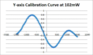
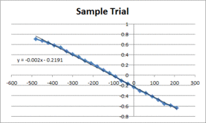
6. Using some form of plotting software (excel was used for analysis of these data), plot the voltage signal versus position. You should get a graph similar to figure 1. An important feature to notice is the linear portion in the middle of the graph. Isolate this portion of the graph by cropping out all of the other points. You should now have a graph that looks similar to figure 2. Fit this graph with a line. The absolute value of the slope of that line is the position calibration for that axis and power level in V/nm.
7. Run the Position Calibration VI for the same power level and axis 5 times on 5 different stuck beads to ensure accuracy.
8. Repeat the calibration for the opposite axis
9. Repeat for multiple power levels (5 different power levels were used for our position calibrations)
10. For each axis and power level, plot the average calibration value over all trials for a specific power level (in V/nm) versus the power level. Generate a line of best fit so that you can determine the calibration value for any power level or axis (if the position calibrations were done extremely carefully, the data should resemble a line). The results of our position calibrations can be seen in the results section.
Possible Sources of Error
1. Accuracy of picomotor travel (for this experiment, the stage movement for this calibration was not 100% unidirectional) 2. Focus of bead - since the beads can't be trapped, we don't know if they are in the center of the trap with respect to the z-axis. This could affect the voltage signal.
Results
| ThorLabs OTKB | 20.309 | |
|---|---|---|
| X position | TBD | 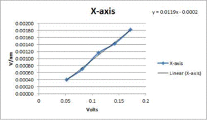
|
| Y position | TBD | 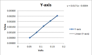
|
Trap stiffness
The force calibrations determine the stiffness of the trap. The stiffness of the trap characterizes the forces exerted by it. Three different methods were used in order to determine the stiffness of each trap: Equipartition, noise PSD roll-off, and Stokes drag.
Methodology
Equipartition
For small displacements from the center of the trap, the trap is considered to be like a spring. The Equipartition method of calculating trap stiffness centers around relating the variance in a trapped object's position due to thermally induced position fluctuations. From the Equipartition Theorem, every degree of freedom in a harmonic potential will contain $ \frac{1}{2} k_B T $ of energy, where $ k_B $ is Boltzmann's constant and T is the absolute temperature. Since the trap acts as a spring, we can equate this energy to the potential energy stored in the 'spring': $ \frac{1}{2} \alpha \left \langle \Delta x^2 \right \rangle $, where $ \alpha $ is the trap stiffness and $ \left \langle \Delta x^2 \right \rangle $ is the variance in position. Solving for $ \alpha $, we get: $ \alpha = \frac{k_B T}{\left \langle \Delta x^2 \right \rangle} $. Assuming these experiments are being run at room temperature, this equation simplifies to: $ \alpha = \frac{4.1124*10^-21}{\left \langle \Delta x^2 \right \rangle} $. Thus, in order to solve for the trap stiffness, the variance in position is the only thing that needs to be calculated. However, since this variance is measured in volts, position calibrations will be required in order to convert the voltage signal into a position in meters (note: since the calibration values from the previous section were in V/nm, you will need to convert these into V/m in order to solve for $ \alpha $). The next section will explain the procedure used to perform this force calibration.
Procedure
1. Using the methods discussed in the Position Calibration procedure, make a slide and load a 1:50,000 dilution of 10% wt stock beads (1 μm silica, Bangs, SS03N/4669) in its channel.
2. Load the slide onto the microscope and trap a bead. Raise the bead to the middle of the slide and move it away from any obstructions. Open the QPD Alignment Tester VI and make sure that the voltage signal is centered at 0 (if it is not, adjust the screws on the QPD so that the signal rests at 0)
3. Open the WriteXYTraceToFile VI. Select which channel you would like to sample from (for this experiment, dev1/ai0 corresponded to the X-axis and dev1/ai1 corresponded to the Y-axis). Enter the Sampling rate in Hz and the sampling time in seconds (for this experiment, 64000 and 3 were used respectively). Start the VI. While the VI is running, carefully watch the IC capture of the slide to make sure that neither the bead leaves the trap nor something else becomes trapped. If either of these things happen, you should discard the data for that trial.
4. Save the data, and load them into an analysis software (Matlab was used for this experiment). Using this software, calculate the variance of the data. The answer given will be in Volts. In order to convert this to meters, divide by your calibration factor squared (NOTE: THE CALIBRATION FACTOR NEEDS TO BE IN V/M AND NOT V/NM AS YOU MEASURED IT!). Finally, using the equation stated in the introduction to this method, calculate your trap stiffness. This answer will be in Newtons per Meter. Since trap stiffnesses are usually measured in picoNewtons per nanoMeter, multiply your result by 1000 to get the right magnitude for those units.
5. As with the position calibration, make sure you run multiple trials for each axis and power level and average the results (depending on the variance of your results, you may wish to take the median of all trials instead of the mean).
6. For each axis and power level, plot the trap stiffness versus the power level. Fit these data to a line. If this calibration and the position calibration were done carefully, the linear fit should be quite accurate.
Possible Sources of Error
1. This calibration requires extremely accurate position calibrations in order to yield accurate data
2. This calibration is very sensitive to noise.
Results
Equipartition
| ThorLabs OTKB | 20.309 | |
|---|---|---|
| X and Y axes | TBD | 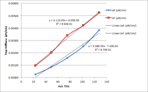
|
