Difference between revisions of "Spring 2020 Assignment 9"
MAXINE JONAS (Talk | contribs) (→The Frequency Dependence of Osmo-Adaptation in Saccharomyces cerevisiae) |
Juliesutton (Talk | contribs) (→The Frequency Dependence of Osmo-Adaptation in Saccharomyces cerevisiae) |
||
| Line 138: | Line 138: | ||
|} | |} | ||
</center> | </center> | ||
| + | |||
| + | Unfortunately, we won't be collecting our own data in the lab this semester, but it's still important to have a feel for what the raw data looks like, and what ''signal'' we are measuring. Download the data file named <tt>'fall2019_StudentData_3.mat'</tt> from the course dropbox folder. This is raw data that was collected by 20.309 students in the Fall of 2019. Load the file into your MATLAB workspace, and you should see a variable called <tt>yeastOsmoticShockData</tt>. This is a struct which contains the movie data, along with some other relevant experimental parameters: | ||
| + | <pre> | ||
| + | >> yeastOsmoticShockData | ||
| + | |||
| + | yeastOsmoticShockData = | ||
| + | |||
| + | struct with fields: | ||
| + | |||
| + | Movie: [544×728×2×32 uint16] | ||
| + | Time: [32×2 double] | ||
| + | ValveState: [32×1 logical] | ||
| + | ValveOscillationPeriod: 480 | ||
| + | BlueCameraGainAndExposure: [3 5000000] | ||
| + | GreenCameraGainAndExposure: [15 5000000] | ||
| + | </pre> | ||
| + | |||
| + | Notice that the movie contains two colors (the third dimension of the movie has a length of 2). The movie matrix is constructed so that the first color represents the GFP-Hog1 signal, and the second color represents the nuclear signal (tagged with RFP). | ||
| + | |||
| + | Use <tt>implay</tt> to watch each color of the movie: | ||
| + | <pre> | ||
| + | implay(double(yeastOsmoticShockData.Movie(:,:,1,:))/4095); | ||
| + | implay(double(yeastOsmoticShockData.Movie(:,:,2,:))/4095); | ||
| + | </pre> | ||
| + | Do they behave as you would expect? | ||
| + | |||
| + | {{Template:Assignment Turn In|message = | ||
| + | # Step through the frames of the movie using the implay controls. Identify a frame where the signal is "high" - in other words, where the Hog1 signal is localized in the nucleus. Turn in the frame number that you've identified and a screen shot of the GFP-Hog1 movie at that frame number. | ||
| + | # Repeat for a frame where the signal is "low" - in other words, where the Hog1 signal is uniformly distributed throughout the cell. Turn in the frame number that you've identified and a screen shot of the GFP-Hog1 movie at that frame number. | ||
| + | }} | ||
| + | |||
{{Template:20.309 bottom}} | {{Template:20.309 bottom}} | ||
Revision as of 14:25, 28 April 2020
Signals and systems
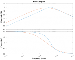
| System function | $ \frac{1}{s+1} $ | $ \frac{s}{s+1} $ | $ \frac{s}{s^2+2s+1} $ | $ \frac{s}{s^2+0.1s+1} $ | $ \frac{1}{s^2+10s+1} $ |
|---|---|---|---|---|---|
| Magnitude plot | |||||
| Phase plot | |||||
| Step response | |||||
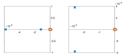
| Pole/zero plot | |||||
| Description |
Magnitude Plots
Phase Plots
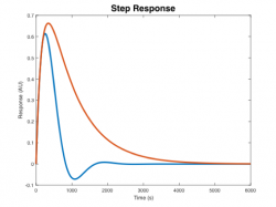
Step Response Plots
Pole Zero Plots
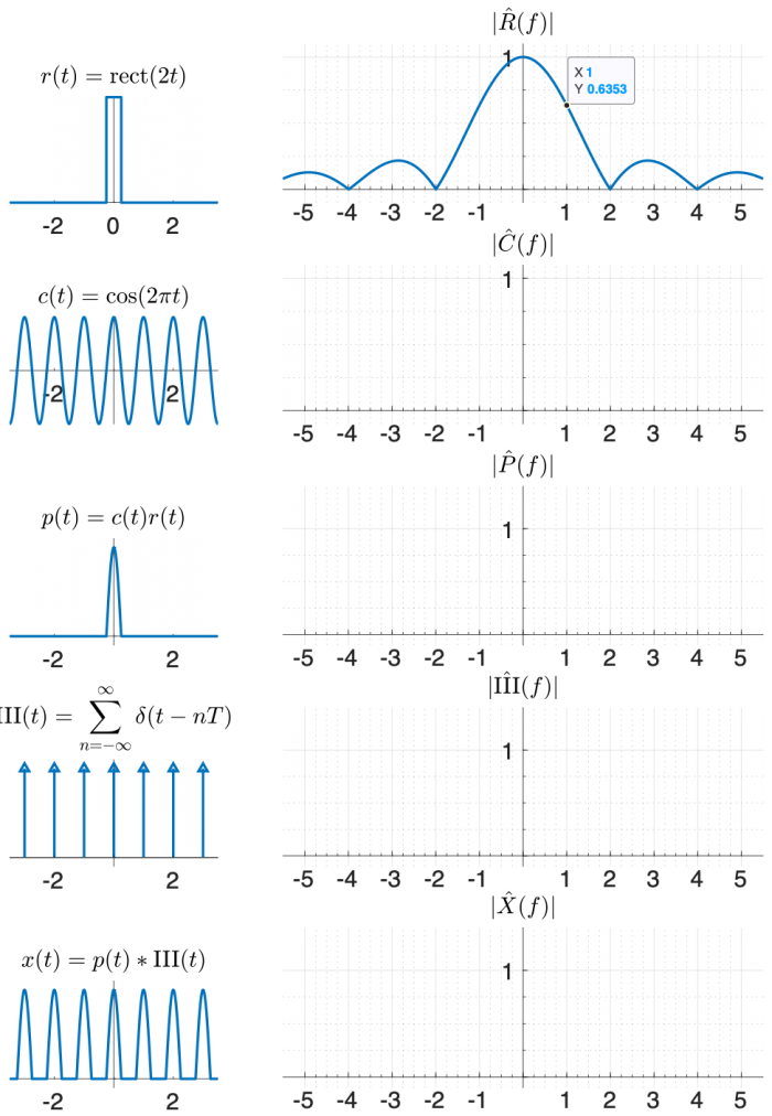
 One way to create x(t) using functions that appear on the transform table is:
- multiply a cosine by a rectangle, and then
- convolve the result with the comb function $ \mathrm{III(}t)=\sum\limits_{n=-∞}^{∞} \delta(t-nT) $.
Use the diagram below to help you find the answer. The left column of shows signals in the time domain, and the right column shows the magnitude of the Fourier transform of each signal. The top right plot is filled in for you, plus a little hint that might help you make an accurate plot.
(The phase of the transforms in this problem is zero at all frequencies, so it is not plotted.)
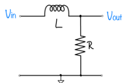
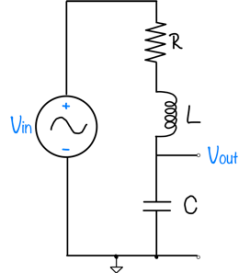
Feedback systems
|

|
The Frequency Dependence of Osmo-Adaptation in Saccharomyces cerevisiae
| |
Read The Frequency Dependence of Osmo-Adaptation in Saccharomyces cerevisiae and the supporting information.. This paper will be the focus of exam 2. We will discuss the paper and the supporting information on Thursday and Friday (4/30 and 5/1). Answer the following questions about The Frequency Dependence of Osmo-Adaptation in S. cerevisiae:
</div> |
|
|
|
Unfortunately, we won't be collecting our own data in the lab this semester, but it's still important to have a feel for what the raw data looks like, and what signal we are measuring. Download the data file named 'fall2019_StudentData_3.mat' from the course dropbox folder. This is raw data that was collected by 20.309 students in the Fall of 2019. Load the file into your MATLAB workspace, and you should see a variable called yeastOsmoticShockData. This is a struct which contains the movie data, along with some other relevant experimental parameters:
>> yeastOsmoticShockData

yeastOsmoticShockData =

  struct with fields:

                         Movie: [544×728×2×32 uint16]
                          Time: [32×2 double]
                    ValveState: [32×1 logical]
        ValveOscillationPeriod: 480
     BlueCameraGainAndExposure: [3 5000000]
    GreenCameraGainAndExposure: [15 5000000]
Notice that the movie contains two colors (the third dimension of the movie has a length of 2). The movie matrix is constructed so that the first color represents the GFP-Hog1 signal, and the second color represents the nuclear signal (tagged with RFP).
Use implay to watch each color of the movie:
implay(double(yeastOsmoticShockData.Movie(:,:,1,:))/4095);
implay(double(yeastOsmoticShockData.Movie(:,:,2,:))/4095);
Do they behave as you would expect?


