Difference between revisions of "Spring 2020 Assignment 8"
(→Convolution practice) |
|||
| Line 1: | Line 1: | ||
{{Template: 20.309}} | {{Template: 20.309}} | ||
| + | ==Circuit analogies== | ||
| + | {{Template:Assignment Turn In|message= | ||
| + | For each of the systems below, find an analogous circuit. | ||
| + | }} | ||
| + | |||
| + | <gallery> | ||
| + | File:Thermal System Analogy Problem.png |Thermal system:Coffee in a thermos | ||
| + | File:Mechanical System Analogy Problem.png|Mechanical system: mass and damper | ||
| + | </gallery> | ||
| + | |||
==Convolution practice== | ==Convolution practice== | ||
{{Template:Assignment Turn In|message= | {{Template:Assignment Turn In|message= | ||
| Line 35: | Line 45: | ||
|} | |} | ||
| − | == | + | |
| − | {{Template:Assignment Turn In|message= | + | ==Fourier transform table== |
| − | + | The two tables below show important properties of the Fourier transform and several useful transform pairs. You can use the tables of pairs and properties to figure out the transforms of an endless number of functions. | |
| + | |||
| + | [[Image: FourierTransformsTable.png|thumb|left|500 px|<caption>Short table of Fourier transform properties</caption>]] | ||
| + | [[Image: TimeFrequencyDomains_MoreTransformPairsTable.png|thumb|left|500 px|<caption>Short table of Fourier transform pairs</caption>]] | ||
| + | |||
| + | {{Template:Assignment Turn In|message= | ||
| + | <ol type="A"> | ||
| + | <li>Sketch each function in table of transform pairs as well as the magnitude of its Fourier transform. Show relevant constants (for example: ''a'', <math>\alpha</math>, and <math>f_0</math>).</li> | ||
| + | <li>Sketch the transform of <math>\cos^4(\omega_0 t)</math>.</li> | ||
| + | <li>Sketch the fourier transform of <math>e^{-\alpha t} u(t) \times \cos(\omega_0 t)</math>. Assume <math>\alpha\ll\omega_0</math>.</li> | ||
}} | }} | ||
| − | + | The table below shows plots of eight time-domain signals A-H. The table on the right includes magnitude plots of the Fourier transform of ten signals numbered 1-10. Some of the frequency plots are shown on log-log axes and some are linear, as indicated by the plot title. | |
| − | + | ||
| − | + | [[Image: PSet4_ConvolutionImage.png|thumb|center|500 px|<caption>Table 8.0.3</caption>]] | |
| − | </ | + | |
| − | {{:Assignment | + | {{Template:Assignment Turn In|message= |
| + | For each time domain signal A-H, write the number 1-10 in the empty column of the matching frequency-domain signal. You may use a numbered plot more than once. | ||
| − | + | ''Hint:'' Gaussian or white noise is a random signal with equal contributions from ''every frequency''.}} | |
{{Template: 20.309 bottom}} | {{Template: 20.309 bottom}} | ||
Revision as of 03:10, 23 April 2020

Circuit analogies
| |
For each of the systems below, find an analogous circuit. |
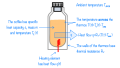
Thermal system:Coffee in a thermos
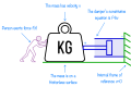
Mechanical system: mass and damper


Convolution practice
| |
For each of the pairs of functions below, plot the convolution of the two functions, $ Y=A*B $ |
| A | B | Y |
|---|---|---|
%2Bdelta(t-1).png)
|
|

|
|
|
 ] ]
|
|
|
|

|
|
|
|
|
|
|
|

|
|
.png)
|
|
|
Fourier transform table
The two tables below show important properties of the Fourier transform and several useful transform pairs. You can use the tables of pairs and properties to figure out the transforms of an endless number of functions.
| |
</div> |
The table below shows plots of eight time-domain signals A-H. The table on the right includes magnitude plots of the Fourier transform of ten signals numbered 1-10. Some of the frequency plots are shown on log-log axes and some are linear, as indicated by the plot title.

| |
For each time domain signal A-H, write the number 1-10 in the empty column of the matching frequency-domain signal. You may use a numbered plot more than once. Hint: Gaussian or white noise is a random signal with equal contributions from every frequency. |