Measuring biological forces mini-lab
Overview
The ability of biological systems to generate and bear mechanical forces is fundamental to an incredibly wide range of processes — obvious activities like muscle contraction and cell motility, but also to more unexpected processes like long term memory, cancer metastasis, and cell division. Exerting and measuring forces at the cellular, sub cellular, and even molecular scale is fundamentally important in many biological research and engineering applications. Two of the most frequently used instruments in these kinds of studies are laser tweezers and atomic force microscopes. In this lab, you will learn how to make quantitative measurements with both of these instruments and discover what ultimately limits their capabilities. If you have time, there are some really cool optional lab activities available, such as Characterizing the e. coli flagellar motor, dna tethers, measuring elastic modulus by micro indentation, or imaging with the AFM.
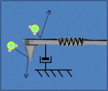
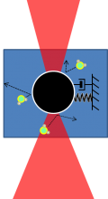
AFM and optical trap model

|

|

|
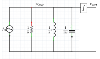
| RLC circuit model of AFM excited by collisions with air molecules. The integrator converts velocity to position. | ||
The circuit model of the AFM and optical trap shown on the right includes a white-noise force source driving a mass, spring, and damper in parallel. (The parallel connection indicates that all of these model components have the same velocity.) The transfer function of the circuit model is:
- $ \frac{x_{out}}{f_{in}}=\frac{\frac{1}{m}}{s^2+\frac{b}{m}s+\frac{k}{m}} $
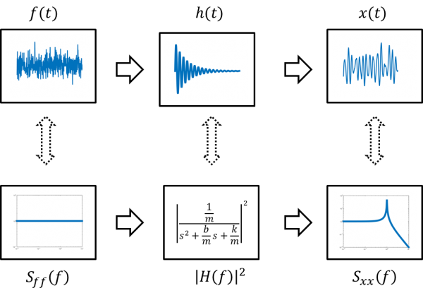
In the time domain, random force input $ f(t) $ drives a second-order system to produce position output $ x(t) $.
The driving force has a constant power spectrum $ P_{ff}=\frac{2K_BT}{\pi^2\Beta} $. The output power spectrum $ P_{xx}(f) $ is equal to the input spectrum times the magnitude of the transfer function squared.

