Difference between revisions of "Exam 2 study guide"
(→Impedance) |
|||
| Line 95: | Line 95: | ||
File:Bode plot low-pass filter example.png|Bode plot low-pass filter example | File:Bode plot low-pass filter example.png|Bode plot low-pass filter example | ||
</gallery> | </gallery> | ||
| + | |||
===Fourier transform=== | ===Fourier transform=== | ||
* The transform takes a signal <math>x(t)</math> as an input and produces a function <math>\hat{X}(\omega)</math> that specifies the amplitude and phase of each complex exponential needed to recreate the signal. | * The transform takes a signal <math>x(t)</math> as an input and produces a function <math>\hat{X}(\omega)</math> that specifies the amplitude and phase of each complex exponential needed to recreate the signal. | ||
| Line 106: | Line 107: | ||
* The impulse response of a system is the output of the system in response to the input <math>x(t)=\delta(t)</math>, where <math>\delta(t)</math> is the Dirac delta function. | * The impulse response of a system is the output of the system in response to the input <math>x(t)=\delta(t)</math>, where <math>\delta(t)</math> is the Dirac delta function. | ||
* ''The imputse response is the Fourier transform of the transfer function''. | * ''The imputse response is the Fourier transform of the transfer function''. | ||
| + | * The transfer function is only one way to represent a system. Other forms include: | ||
| + | ** Impulse response. (Transfer function is the inverse Fourier transform of <math>h(t)</math>) | ||
| + | ** Single differential equation. (Trivial to find from transfer fountain — cross multiply and replace <math>s</math> with <math>d/{dt}</math>. | ||
| + | ** Poles, zeros, and gain. | ||
| + | *** Zeros are values of s for which the numerator of the transfer function goes to zero | ||
| + | *** Poles are values of s where the denominator | ||
| + | *** Factor the numerator and denominator to convert a transfer function to poles and zeros. | ||
| + | *** You can show the poles and zeros on a ''pole zero plot'' with x's in the locations of the poles and o's in the location of the zeros. | ||
| + | |||
<gallery> | <gallery> | ||
File:Signals and systems overview.png|Signals and systems overview | File:Signals and systems overview.png|Signals and systems overview | ||
File:Convolution integral.png|Convolution integral | File:Convolution integral.png|Convolution integral | ||
File:Transform of low-pass transfer function.png|Example: low-pass transfer function | File:Transform of low-pass transfer function.png|Example: low-pass transfer function | ||
| + | File:Pole zero plot of a low-pass filter.png|Pole zero plot of a low-pass filter | ||
</gallery> | </gallery> | ||
| Line 120: | Line 131: | ||
File:Cascade pattern bottom line.png|Cascade pattern bottom line | File:Cascade pattern bottom line.png|Cascade pattern bottom line | ||
</gallery> | </gallery> | ||
| + | |||
| + | ===Second order system=== | ||
| + | * A second-order system includes two capacitors or two inductors or one capacitor and one inductor. | ||
| + | * Second order system | ||
| + | ** Characteristic polynomial | ||
| + | ** Damping ratio, undamped natural frequency, undamped natural frequency | ||
| + | <gallery> | ||
| + | File:Parallel RLC circuit.png|Parallel RLC circuit | ||
| + | </gallery> | ||
| + | |||
===Feedback systems/Black's formula=== | ===Feedback systems/Black's formula=== | ||
* In a feedback system with forward transfer function <math>A(s)</math> and feedback transfer function <math>\Beta(s)</math>, the overall transfer function <math>H(s)=\frac{V_{out}}{V_{in}}=\frac{A(s)}{1+\Beta(s)A(s)}</math> | * In a feedback system with forward transfer function <math>A(s)</math> and feedback transfer function <math>\Beta(s)</math>, the overall transfer function <math>H(s)=\frac{V_{out}}{V_{in}}=\frac{A(s)}{1+\Beta(s)A(s)}</math> | ||
| Line 127: | Line 148: | ||
</gallery> | </gallery> | ||
| − | |||
| − | |||
| − | |||
| − | |||
| − | |||
| − | |||
| − | |||
| − | |||
Things you should know: | Things you should know: | ||
Revision as of 15:18, 7 May 2019


Optics
You should understand every component of the two-color microscope design: what it does, where it goes, which direction it faces, and key performance specifications (focal length, spectrum, ...).
- fluorophores
- excitation and emission spectra
- extinction coefficient
- quantum yield
- lenses
- focal length
- placement
- orientation
- model of objective lens
- filters
- excitation
- dichroic
- emission
- light sources
- spectrum
- optical model
- CMOS camera
- optimal pixel size
Circuits, signals, and systems
Electrical circuit quantities and units
- The state variables for electronic circuits are voltage and current.
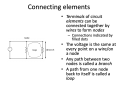
- One way to specify a circuit model is to draw a network of ideal elements connected by ideal wires.
- A node consists of two or more element terminals connected together by an ideal wire. All terminals connected to the node have the same voltage.
- A branch is a path between two nodes.
- A path from one node back to itself is a loop.
- One node, called the ground node, is defined to have a voltage $ V=0 $. This node is sometimes indicated by a triangular ground symbol.
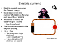
Electrical current units
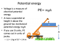
Electrical potential energy
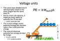
Voltage units
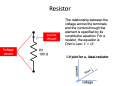
Resistor symbol and constitutive equation
Basic ideal circuit elements
Anatomy of a circuit diagram


Conservation laws, circuit patterns
- The primary method for finding node voltages and branch currents in a circuit model is to apply the current conservation law on nodes and the voltage conservation law on loops in conjunction with the constitutive equations of the elements connected to a node or transited in a loop.
- Current conservation law: the sum of currents flowing into a node is equal to zero.
- Voltage conservation law: the sum of voltages around a loop is equal to zero.
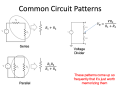
- Knowing a few common patterns can dramatically simplify analysis of many circuit models.
- Two elements in series have the same current. The equivalent impedance of elements in series is $ Z_{eq}=\sum{Z_i} $.
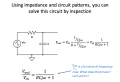
- Two elements in parallel have the same voltage. The equivalent impedance of elements in parallel is $ \frac{1}{Z_{eq}}=\sum{\frac{1}{Z_i}} $.
- In a voltage divider, $ V_{out}=V_{in}\frac{Z_2}{Z_1+Z_2} $
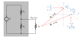
- For a two-terminal circuit including any number of elements, you can create a Thevenin equivalent circuit that includes only one voltage source and one resistor (or impedance).
- $ V_{oc}=I_{sc}R_{eq} $, where $ V_{oc} $ is the open circuit voltage, $ I_{sc} $ is the short circuit current, and $ R_{eq} $ is the equivalent resistance.
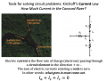
Kirchoff's current law
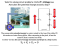
Kirchoff's voltage law
Common circuit patterns
Thevenin equivalent circuit.


Impedance
- The electrical impedance (𝑍) of an element is equal to its voltage divided by current, assuming voltage has the form $ Z=V/I $.
- Impedance is a measure of resistance to electrical flow.
- High impedance means that little current flows for a given voltage.
- Low impedance means the opposite.
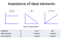
- The impedance of a resistor is the constant quantity $ R $.
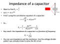
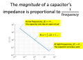
- The impedance of a capacitor is a function of frequency: $ Z_C=\frac{1}{Cs} $, where $ s=j\omega $.
- The impedance of a capacitor goes to infinity as $ \omega\rightarrow0 $. At low frequencies, a capacitor looks like an open circuit.
- The impedance of a capacitor goes to zero as $ \omega\rightarrow\infty $. At high frequencies, a capacitor looks like a wire or short circuit.
- The impedance of an inductor is $ Z_L=Ls $.
- The impedance of an inductor goes to zero as $ \omega\rightarrow0 $. At low frequencies, an inductor looks like a wire or short circuit.
- The impedance of an inductorr goes to infinity as $ \omega\rightarrow\infty $. At high frequencies, an inductor looks like an open circuit.
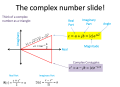
Complex numbers
Impedance of a capacitor
Capacitor impedance vs frequency plot
Impedance of the ideal elements


Signals and systems definitions
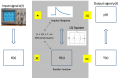
- A signal is a mathematical function that represents information such as how voltage varies over time or the pattern of light intensity over space.
- A system operates on one or more signals and produces an output.
- A subset of systems, called LSI systems, exhibit the properties of linearity and shift invariance.
- In an LSI system, a sinusoidal input of frequency ω will generate an output that is a sinusoid of the same frequency, possibly with its magnitude scaled and its phase shifted (offer).
Transfer functions and Bode plots
- The transfer function of an LSI system is equal to the ratio of its input signal divided by its output signal: $ H(s)=\frac{V_{out}}{V+{in}} $, assuming the input signal has the form $ V_{in}=e^{st} $
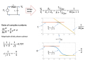
- You can make a type of system called a low-pass filter by connecting one resistor and one capacitor in a voltage divider configuration, with the capacitor on the "bottom".
- It's easy to find the transfer function of a low-pass filter using the divider pattern: $ H(s)=\frac{1/{Cs}}{R+{1/{Cs}}}=\frac{1}{RCs+1} $
- One way to visualize the transfer function is to plot its magnitude and phase as a function of frequency (Bode plot).
- Magnitude is normally plotted on log-log axes.
- Phase is normally plotted on semi-log axes.
- The plot graphically shows the scale factor and phase shift that each sinusoid undergoes as a function of frequency

Transfer functions
Solving the low-pass filter with voltage divider pattern
The Bode plot slide!
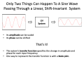
Sinusoids through an LSI system.
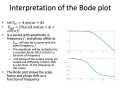
Interpretation of Bode plots
Bode plot low-pass filter example


Fourier transform
- The transform takes a signal $ x(t) $ as an input and produces a function $ \hat{X}(\omega) $ that specifies the amplitude and phase of each complex exponential needed to recreate the signal.
- The definition of the transform is: $ \hat{X}(f)=\int_{-\infty}^{\infty}x(t)e^{-2\pi j f t}dt $
- The Fourier transform table show transform pairs of many functional forms as well as properties of the transform
Convolution theorem, impulse response, and transfer function
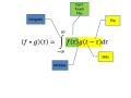
- Convolution and multiplication are dual operations in the time and frequency domain. If you convolve one signal with another, you multiply their transforms. If you multiply two signals, their transfers convolve.
- You can convolve two signals graphically using the "flip, slide, multiply, integrate" method.
- If the input to a linear system is $ x(t) $, then the output is $ y(t)=x(t)*h(t) $, where $ h(t) $ is the impulse response of the system.
- The impulse response of a system is the output of the system in response to the input $ x(t)=\delta(t) $, where $ \delta(t) $ is the Dirac delta function.
- The imputse response is the Fourier transform of the transfer function.
- The transfer function is only one way to represent a system. Other forms include:
- Impulse response. (Transfer function is the inverse Fourier transform of $ h(t) $)
- Single differential equation. (Trivial to find from transfer fountain — cross multiply and replace $ s $ with $ d/{dt} $.
- Poles, zeros, and gain.
- Zeros are values of s for which the numerator of the transfer function goes to zero
- Poles are values of s where the denominator
- Factor the numerator and denominator to convert a transfer function to poles and zeros.
- You can show the poles and zeros on a pole zero plot with x's in the locations of the poles and o's in the location of the zeros.
Signals and systems overview
Convolution integral
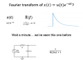
Example: low-pass transfer function
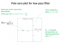
Pole zero plot of a low-pass filter


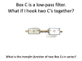
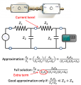
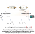
Cascade pattern
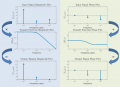
- The transfer functions of two systems connected in a cascade multiply if $ Z_{out} $ of the first system is much less than $ Z_{in} $ of the second system.
Cascade pattern
Cascade pattern "extra term"
Cascade approximation
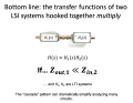
Cascade pattern bottom line


Second order system
- A second-order system includes two capacitors or two inductors or one capacitor and one inductor.
- Second order system
- Characteristic polynomial
- Damping ratio, undamped natural frequency, undamped natural frequency
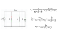
Parallel RLC circuit

Feedback systems/Black's formula
- In a feedback system with forward transfer function $ A(s) $ and feedback transfer function $ \Beta(s) $, the overall transfer function $ H(s)=\frac{V_{out}}{V_{in}}=\frac{A(s)}{1+\Beta(s)A(s)} $
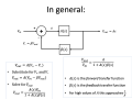
Black's formula
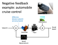
Negative feedback cruise control


Things you should know:
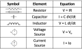
- Ideal LSI circuit elements (resistor, capacitor, inductor, voltage source, current source)
- symbol
- constitutive equation
- Voltage/current conservation laws
- Series and parallel patterns
- Divider pattern
- Impedance
- Equivalent circuits
- First-order low- and high-pass filters
Signals and systems
- Equivalent representations of an LSI system
- Single differential equation
- Poles and zeros
- Coupled differential equations
Feedback systems
- Black’s formula
- Effect of gain on feedback response
- Root locus diagram
Mettetal paper

Simplified osmotic shock story
You should understand the basic story of how S. cerevisiae recovers from osmotic shock. You don’t need to memorize the specific proteins involved.
Key points (not all of which are in the Mettetal paper):
- Osmosis is a thing:
- The cell membrane is permeable to water, but not to most everything else. (Other molecules enter or leave via membrane transport proteins.)
- Water molecules move across the cell membrane in the direction from low to high osmotic concentration.
- Osmotic pressure does not depend on the identity of the solute molecules – only their molar concentration.
- Dictionary definition of osmosis: A process by which molecules of a solvent tend to pass through a semipermeable membrane from a less concentrated solution into a more concentrated one, thus equalizing the concentrations on each side of the membrane.
- At equilibrium, glycerol leaves S. cerevisiae via a membrane transport channel.
- The aquaglyceroporin Fps1 is maintained in open state by a protein called Rgc2 bound to its C-terminal.
- Increasing the extracellular salt concentration causes water to leave the cell.
- The cell shrinks and the hydrostatic pressure on the cell membrane decreases.
- Osmosensor proteins detect reduced turgor pressure (the force from within the cell that pushes on the cell wall) and activate the mitogen-activated protein kinase (MAPK) Hog1.
- The osmosensors activate two redundant signaling pathways. Both pathways converge on the MAPKK protein Pbs2. In other words, Pbs2 activates Hog1.
- Activated Hog1 initiates a several of actions that increase the glycerol concentration in the cell
- Hog1 stops glycerol efflux by phosphorylating/evicting Rgc2 from Fps1.
- Activated Hog1 enters the nucleus, where it upregulates two proteins involved in the production of glycerol, Gpd1 and Gpp2 (among other things such as arresting the cell cycle and upregulating Stl1)
- Hog1 gets deactivated in the nucleus and exported to the cytoplasm
System model
Activated Hog1 enters the nucleus. • “We applied system identification methods to infer a concise predictive model.” • “We found that the dynamics of the osmo-adaptation response are dominated by a fast-acting negative feedback through the kinase Hog1 that does not require protein synthesis.”
Experiment and analysis
Cite error: <ref> tags exist, but no <references/> tag was found