DNA Melting: Simulating DNA Melting - Intermediate Topics

Introduction

This tutorial will show you how to simulate the DNA melting experiment in Matlab. It will be essential to have your data analysis scripts working before you come to the lab. You can use a simulated dataset to help debug your data analysis scripts. You can copy the code from this tutorial and paste it into a Matlab command window.

In the DNA Melting Lab, the raw data you will record consists of two voltages that vary over time. In order to estimate the melting temperature, these raw voltages will have to be converted to a melting curve, which gives the fraction of dsDNA as a function of temperature. T_m can be estimated directly from the melting curve or by finding the peak of the melting curve's derivative.

Data analysis steps include:

1. Filter raw data to remove noise.
2. Transform RTD voltage to temperature.
3. Transform photodiode current to relative fluorescence.
4. Ensure that the melting function is uniquely values by combining samples with identical temperature values.
5. Differentiate the resulting function.

Before you begin

• If you need a review of Matlab fundamentals, see Matlab:Matlab Fundamentals
• Read the DNA Melting Lab Manual.
• You may also find it helpful to review the DNA Melting Thermodynamics Lecture Notes.

Simulating DNA melting

Model cooling of the sample

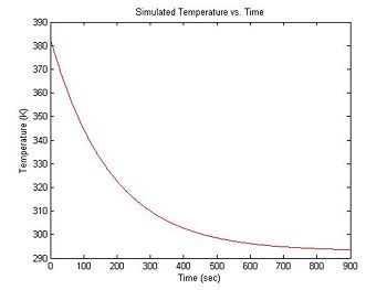
At the beginning of an experimental run, the DNA + fluorescent dye sample is heated in a bath to around 90°C. Over a period of about 15 minutes, the sample cools to room temperature (about 20°C). Cooling can be approximated by an exponential function with a time constant of 3 minutes. Thus, the equation for temperature (in °K) versus time is:

$ T(t) = 90 e ^ {-\frac{t}{180}} + 293 $

In Matlab:

simulationLength = 900                  % 15 minute simulation
sampleRate = 1                          % 1 Hz sample rate
t = 0:(1/sampleRate):simulationLength;  % create a time vector (units: seconds)
T = 90 * exp(-1 * t / 180) + 293;       % exponential cooling from 383K to 293K
plot(t, T, 'r');
xlabel('Time (sec)');
ylabel('Temperature (K)');
title('Simulated Temperature vs. Time');

Remember that the semicolon at the end of the line prevents Matlab from displaying dozens of annoying lines on the console containing the value of t.

Convert sample temperature to Voltage

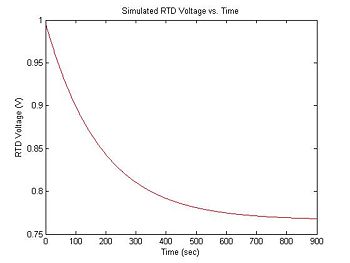
The RTD device does not measure temperature directly. The resistance of the RTD is $ R_{RTD} = 1000 + 3.85(T - 273) $. In the experimental apparatus, the RTD is hooked up as a voltage divider with another resistor, R. The power supply is 15 volts. Thus, the output voltage is: $ V_{RTD} = 15 * R_{RTD}/(R + R_{RTD}) $. The following code converts the tepmerature vector T into the equivalent RTD voltage measurements, assuming R = 20KΩ. The resulting graph should be similar to what you measure in the lab.

R_RTD = 1000 + 3.85 * (T - 273);           % Compute RTD resistance in Ohms
V_RTD = 15 * R_RTD ./ (20E3 + R_RTD);      % Compute V_RTD in Volts
plot(t, V_RTD, 'r');
xlabel('Time (sec)');
ylabel('RTD Voltage (V)');
title('Simulated RTD Voltage vs. Time');

Add some noise

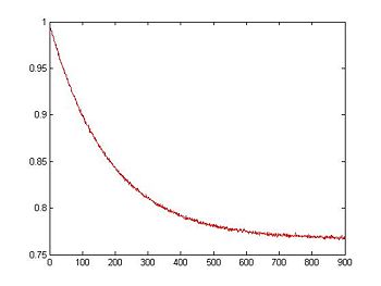
You will certainly notice some noise on the signals you capture. (See: Where does electonic noise come from?.) To simulate that, we can use Matlab's randn function, which generates normally distributed random numbers. Noise will be an extremely important (and annoying) factor in this experiment because the melting curve must be differentiated. Differentiation emphasizes noise. (Think about the frequency response of a differentiator.)

noise = 0.001 * randn(1,length(V_RTD));    % Create Gaussian noise signal with standard deviation 1 mV
V_RTD = V_RTD + noise;                     % Add simulated noise to the voltage signal
plot(t, V_RTD, 'r');
xlabel('Time (sec)');
ylabel('RTD Voltage (V)');
title('Simulated RTD Voltage with Noise vs. Time');

Write a function to compute f

The first useful piece of code is a function that will compute $ \left . f \right . $ from the equation derived in class. This function must be in its own file called DnaFraction.m.

<include src="http://web.mit.edu/~20.309/www/Matlab/DnaFraction.m" />

The element-by-element divide operator (./) is used instead of the matrix divide operator(/) so that the temperature parameter T can be a vector. If T is a single value, both operators are equivalent. But the / operator will try to do a matrix divide if T is a vector or matrix and give an error since the dimension of the two operands do not match. A for...end loop could also be used to call DnaFraction once for each value of $ T $. But for loops have terrible performance in Matlab and your program will run much faster if you use a vector of $ T $ values instead.

%Returns the fraction of dsDNA given total DNA concentration, temperature, Delta S, and Delta H
%Usage: f = DnaFraction(Ct, T, DeltaS, DeltaH)
function f = DnaFraction(Ct, T, DeltaS, DeltaH)

%Constants
R=8.3;

%first compute Ct * Keq
CtKeq = Ct * exp(DeltaS / R - DeltaH / (R * T));

%now compute f
f = (1 + CtKeq + sqrt(1 + 2 * CtKeq))/CtKeq;

Test the function

First, create a temperature vector. Then call DnaFraction with some reasonable parameters and plot the result. Units are calorie, mole.

t = [20:90] + 273;
f = DnaFraction(.1E-6, t, 304E3, 786);
plot(t,f)