Difference between revisions of "DNA Melting: Simulating DNA Melting - Intermediate Topics"

This page is being revised. To be finalized by October 28th, 2011 -Steven

Add some noise

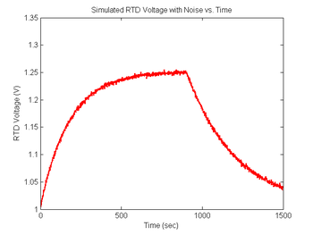
You will certainly notice noise on the signals you capture in the lab. Noise will be an extremely important (and annoying) factor in this experiment because the melting curves will be differentiated. Differentiation emphasizes noise. In order to ensure that your data analysis script effectively handles the noise you are likely to observe, simulated random and impulse noise will be added to the signals.

To simulate noise, we can use Matlab's randn function, which generates normally distributed random numbers with unity standard deviation. The two arguments tell randn to create a vector of random samples with size 1xlength(V_RTD).

noise = 0.001 * randn(1,length(sim1.V_RTD))';    % Create noise vector, standard deviation=1mV
sim1.V_RTD = sim1.V_RTD + noise;                % Add simulated noise to the voltage signal

figure(8)
plot(sim1.time, sim1.V_RTD, 'r');
xlabel('Time (sec)');
ylabel('RTD Voltage (V)');
title('Simulated RTD Voltage with Noise vs. Time');

Revisit your code from DNA Melting: Simulating DNA Melting - Basics and using the approach above add noise to your RTD voltage signal, then explore the behavior of your code for different levels of noise. In particular, you can add differentiation of the curve from Figure 6 and discover the issues with attempts to differentiate that signal without additional processing. You will likely find that you first need to either sort or bin your temperature data so that the f vs T function can be differentiated. Then also run this data through your fit function and observe any difference in the fit statistics.

You are also encouraged to add noise at additional frequencies that you think might be present in the lab, then attempt to filter that data in Matlab to test the effectiveness of the RTD voltage filter design that you built in the lab. To do this, generate the noise (perhaps 60 Hz, pink noise, possibly high frequency noise from switching in the overhead lights, or even noise on the earth ground that could be coming from equipment elsewhere in the building) and add it to the signal from Figure 8. Remember it is a long way to the earth from our lab. Next filter that signal using your transfer function and the matlab command lsim. Then again run this data through your fit function.

Model the sample fluorescence signal

Now that we have a simulated RTD voltage signal, the next step is to simulate the fluorescence signal.

The output range of the transimpedance amplifier depends on many factors, including: dsDNA quantity, illumination intensity, fluorophore efficiency, optical system gain, photodiode efficiency, and electronic amplifier gain. All of the factors except dsDNA concentration essentialy remain constant. Thus, the output of the transimpedance amplifier can be modeled by a single overall system gain factor times the dsDNA fraction. In addition, the amplifier output may be offset by a constant DC value, which is simple to model. (If the output of your apparatus drifts significantly over time, you will need to improve your implementation and methods to minimize this. The suggested design includes a potentiometer for adjusting DC offset.)

Scale the curve and add some noise

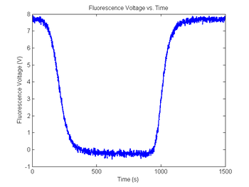
The output range of the transimpedance amplifier over the course of an experimental run can vary depending on several factors, including the amplifier gain, optical system gain, etc... A typical setup might produce values between, say, 0.5 and 7.2 Volts. The simulation code generates two random numbers to set the range and minimum value of the data. Your data analysis script will have to normalize the amplifier output voltage to a fractional value between 0 and 1. (What assumptions will you make about dsDNA concentration to do the normalization?)

In addition to Gaussian noise, the high gain amplifier sometimes produces impulse noise. This can be caused by small static discharges, for example when a charged person sits down in a chair in the lab. It is a good idea to include some filtering for impulse noise in your data analysis script, in case your apparatus is susceptible to impulse noise.

Range = 5 + 4 * rand();                              % Range between 5 and 9
Minimum = 2 * rand() - 1;                            % Minimum between +/- 1
sim1.V_f = Range * sim1.dsDnaFraction + Minimum;     % Scale output
noise = 0.01 * randn(1,length(sim1.V_f))';           % Random noise, standard deviation=10mV
sim1.V_f = sim1.V_f + noise;                         % Add random noise
noise = rand(1,length(sim1.V_f))';                   % Uniformly distributed  random numbers
ImpulseNoiseProbability = 1 ./ 75;                   % Probability of impulse noise
noise = 20 * (noise < ImpulseNoiseProbability) - 10; % Quantize impulse noise
sim1.V_fNoisy = max(sim1.V_f, noise);                     % Add in impulse noise

figure(9)
plot(sim1.time, sim1.V_fNoisy)
title('Fluorescence Voltage vs. Time');
xlabel('Time (s)');
ylabel('Fluorescence Voltage (V)');

Reformat the data

When you import data from the LabView program that records DNA melting data, the format will be an N x 2 matrix with $ V_T $ values in column 1 and $ V_f $ in column 2. To put the simulated data in the same format, you can use Matlab's transpose operator (.') and the horizontal concatenation function horzcat:

simData = horzcat( sim1.V_RTD .', sim1.V_f .');
size(simData)


ans =

   901     2

Please see this page if you are uncertain about the .' operator.

Congratulations. You now have a simulated dataset that should be quite similar to what you measure in the lab.

Improving the model: photobleaching (optional)

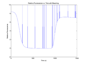
Each time a SYBR Green molecule is excited by a photon, there is a small chance that it will be destroyed and permanently lose its ability to fluoresce. The effect of photobleaching on the measured fluorescence intensity can be significant. To demonstrate this, a model for photobleaching may be added to the simulation. In the model, a small, fixed percentage of the fluorophores are mathematically destroyed each time sample. This simple difference equation can be implemented with a for…end loop.

$ {\hat{f}}_{N} = B {\hat{f}}_{N-1} + f_{N} - f_{N-1} $

where,

$ {\hat{f}}_N $ is the Nth sample of the bleached relative fluorescence,

$ \left . B \right . $ is a bleaching constant equal to the fraction of fluorophore not destroyed per time sample, and

$ \left . f_N \right . $ is the Nth sample of the dsDNA fraction (relative fluorescence) curve.

The fraction of fluorophores destroyed per time sample is set by the variable bleachingConstant. In the example code, the constant is set so that half of the fluorophores will be destroyed over the course of the simulated experimental run.

sim1.filtV_f = medfilt1(sim1.V_fNoisy,15); % temporarily remove shot noise
sim1.fluorescenceNorm = sim1.filtV_f / max(sim1.filtV_f); % normalize photo diode signal to dsDNA fraction
sim1.bleachingCoefficient = 1e-5;              % 1/s, estimated from previous experiments
sim1.bleachingConstant = 1e-4;               % 1/s, estimated from previous experiments
sim1.bleachingCorrection = (1 - sim1.bleachingCoefficient ...
    .* cumsum(1 .* sim1.fluorescenceNorm)) ...
    .* (1 - sim1.bleachingConstant .* (0:(length(sim1.fluorescenceNorm)...
    - 1))');    % calclation of bleaching correction by two methods, exponetial and linear
sim1.fluorescenceBleached = sim1.fluorescenceNorm ...
    .* sim1.bleachingCorrection;
Range = 5 + 4 * rand();                              % Range between 5 and 9
Minimum = 2 * rand() - 1;                            % Minimum between +/- 1
sim1.V_fScaled = Range * sim1.fluorescenceBleached + Minimum;     % Scale output
noise = rand(1,length(sim1.V_fScaled))';                   % Uniformly distributed  random numbers
ImpulseNoiseProbability = 1 ./ 75;                   % Probability of impulse noise
noise = 20 * (noise < ImpulseNoiseProbability) - 10; % Quantize impulse noise
sim1.V_fBleached = max(sim1.V_fScaled, noise);                     % Add in impulse noise

figure(10)
plot(sim1.time, sim1.V_fBleached)
title('Relative Fluorescence vs. Time with Bleaching');
xlabel('Time (s)');
ylabel('Relative Fluorescence');

The value of the first element of the vector sim1.dsDnaFractionBleached sets the initial condition for the difference equation — the relative fluorescence at the beginning of the simulation. Because SYBR green exhibits a small amount of intrinsic fluorescence when it is not bound to dsDNA, the initial value of sim1.dsDnaFractionBleached is set to a small number to model this effect.

Experiment with the bleaching constant and intrinsic fluorescence values to see how they distort the melting curve. Increasing the bleaching constant is equivalent to turning down the illumination intensity: fewer fluorphores will be destroyed in a given time. Unfortunately, the overall fluorescence intensity also decreases, necessitating higher amplifier gain and decreased signal to noise ratio. How will you decide on the optimal illumination and amplification levels in the lab? Can you use this model to correct for photobleaching effects in your data? How can you determine the bleaching constant experimentally?

Follow the steps in the previous section for scaling the relative fluorescence signal, adding noise, and reformatting.