Difference between revisions of "DNA Melting: Simulating DNA Melting - Intermediate Topics"
(→Simulate cooling of the sample) |
(→Simulate cooling of the sample) |
||
| Line 91: | Line 91: | ||
<pre> | <pre> | ||
| − | simulationLength = 900 | + | simulationLength = 900 % 15 minute simulation |
| − | sampleRate = 1 | + | sampleRate = 1 % 1 Hz sample rate |
| − | sim1.time = 0:(1./sampleRate):simulationLength; | + | sim1.time = 0:(1./sampleRate):simulationLength; % create time vector (units: seconds) |
| − | sim1.temperature = 90 * exp(-1 * t ./ 180) + 293; % exponential cooling from 383K to 293K | + | sim1.temperature = 90 * exp(-1 * sim1.t ./ 180) + 293; % exponential cooling from 383K to 293K |
plot(sim1.time, sim1.temperature, 'r'); | plot(sim1.time, sim1.temperature, 'r'); | ||
Revision as of 20:25, 23 April 2008
Contents
Introduction
This tutorial will show you how to simulate the DNA melting experiment in Matlab. It will be essential to have your data analysis scripts working before you begin running experiments in the lab. You can use a simulated dataset generated by the code in this tutorial to help debug your data analysis scripts.
The raw data you will take in the lab consists of periodic measurements of two voltages. The job of your data analysis scripts will be to convert the two voltages into a melting curve, which is a plot of dsDNA fraction versus temperature, and its derivative. From the melting curve, $ \left . T_m \right . $, $ \Delta H^{\circ} $, and $ \Delta S^{\circ} $ for the annealing of several DNA samples will be estimated.
Code from this page can be copied into a Matlab command window. M-files are available in the course locker.
If you prefer to work in Python, please see this page.
Before you begin
- Read the DNA Melting Lab Manual.
- Review the DNA Melting Thermodynamics Notes.
- Review Introduction to Convolution and Digital Filtering.
- If you need a review of Matlab fundamentals, see Matlab Fundamentals tutorial.
Procedure
In outline, the steps to simulate a DNA melting experimental run are:
- Model the DNA annealing reaction
- Model sample cooling versus time
- Compute RTD voltage over time from temperature data
- Add noise to the RTD signal
- Compute relative fluorescence intensity from temperature data
- (Optional) model photobleaching
- Scale the fluorescence intensity signal and add noise
DNA annealing
Write a function to compute the fraction of dsDNA at a given temperature
The dsDNA concentration at a given temperature can be computed with the equation that we derived in class:
- $ K_{eq} = e^\left [\frac{\Delta S^{\circ}}{R} - \frac{\Delta H^{\circ}}{R T} \right ] $
- $ f = \frac{1 + C_T K_{eq} - \sqrt{1 + 2 C_T K_{eq}}}{C_T K_{eq}} $
Since this is a very complicated equation and we will use it many times, it makes sense to write a Matlab function. An m-file containing the code shown here is available online here. Remember that Matlab functions must be saved in your current directory or another directory in the Matlab path. The name of the file must be the function name appended with ".m".
<include src="http://web.mit.edu/~20.309/www/Matlab/DnaFraction.m" />
The DnaFraction function takes an optional fifth argument for the gas constant so that different unit systems can be used. The Matlab function nargin is used to determine whether a fifth argument has been supplied. If not, R is set to the default value of 1.987.
Using the element-by-element divide operator makes it possible for the DnaFraction function to accept either a single value of temperature or a vector of temperature samples. (As a general rule, use the ./ operator instead of / unless you intend to do a matrix divide.)
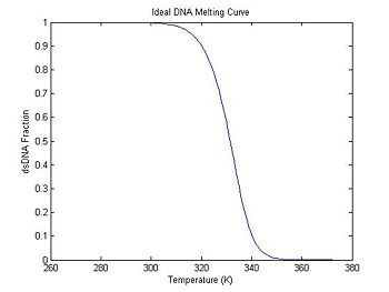
Ideal melting curve
Since DnaFraction can take a vector for its temperature argument, generating a melting curve is simple:
ideal = struct();                                        % create an empty structure
ideal.temperature = 273:372;                             % 100 temperature samples (K)

% DnaFraction arguments: concentration, temp. vector, delta S, delta H, (optional R)
ideal.dsDnaFraction = DnaFraction(1E-6, ideal.temperature, -184, -71E3);

plot(ideal.temperature, ideal.dsDnaFraction);
title('Ideal DNA Melting Curve');
xlabel('Temperature (K)');
ylabel('dsDNA Fraction');
Using the structure ideal allows you to keep the data from several simulations in your workspace without getting them confused.
Derivative of the melting curve
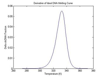
One method of estimating $ T_m $ is to find the temperature where the dsDNA fraction equals 1/2. Another method is to differentiate the melting curve. $ T_m $ occurs at the peak of the derivative — where the dsDNA fraction is changing the fastest.
The Matlab function diff computes the difference of a vector, which is a discrete approximation of the derivative. But there is a problem: the result of diff is one element shorter than the input vector. There are several ways to handle this. The simplest one is shown in the code below, which generates a new temperature vector with values centered between the original temperature samples.
ideal.dTemperature = ideal.temperature(1:99) + 0.5; % create new temperature vector
ideal.dDsDnaFraction = diff(ideal.dsDnaFraction);   % take the difference

plot(ideal.dTemperature, -1 * ideal.dDsDnaFraction);
title('Derivative of Ideal DNA Melting Curve');
xlabel('Temperature (K)');
ylabel('Delta dsDNA Fraction');
Note that the dsDNA fraction equals 0.5 at about 332.5 degrees in the melting curve and the peak of the derivative also occurs at the same temperature. (The curve is poltted inverted.) Why would you prefer one method over the other for estimating the melting temperature from experimental data?
Simulate cooling of the sample
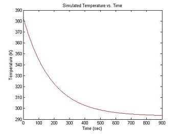
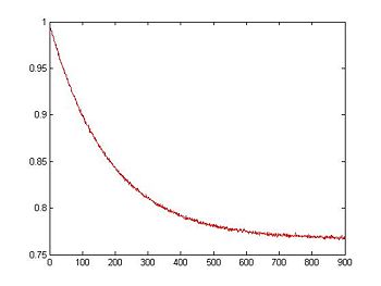
During each experimental run, the range of temperatures will be provided by natural cooling of the sample after it has been heated in a bath. At the beginning of an experimental run, the DNA + fluorescent dye sample is heated in a bath to around 90°C. Over a period of about 15 minutes, the sample cools to room temperature (about 20°C). Cooling can be approximated by an exponential function with a time constant of 3 minutes. The equation for temperature (in °K) versus time is:
- $ T(t) = 90 e ^ {-\frac{t}{180}} + 293 $
In Matlab:
simulationLength = 900                                 % 15 minute simulation
sampleRate = 1                                         % 1 Hz sample rate
sim1.time = 0:(1./sampleRate):simulationLength;        % create time vector (units: seconds)
sim1.temperature = 90 * exp(-1 * sim1.t ./ 180) + 293; % exponential cooling from 383K to 293K

plot(sim1.time, sim1.temperature, 'r');
xlabel('Time (sec)');
ylabel('Temperature (K)');
title('Simulated Temperature vs. Time');
If you have any questions about the element-by-element division operator in Matlab (./) see:this page.
Convert sample temperature to RTD Voltage
Model the voltage divider
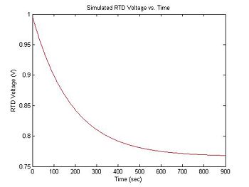
The RTD device does not measure temperature directly. The resistance of the RTD is $ R_{RTD} = 1000 + 3.85(T - 273) $. In the experimental apparatus, the RTD is hooked up as a voltage divider with another resistor, R. The power supply is 15 volts. Thus, the output voltage is: $ V_{RTD} = 15 * R_{RTD}/(R + R_{RTD}) $. The following code converts the temperature vector T into the equivalent RTD voltage measurements, assuming R = 20KΩ.
R_RTD = 1000 + 3.85 * (T - 273);           % Compute RTD resistance in Ohms
V_RTD = 15 * R_RTD ./ (20E3 + R_RTD);      % Compute V_RTD in Volts
plot(t, V_RTD, 'r');
xlabel('Time (sec)');
ylabel('RTD Voltage (V)');
title('Simulated RTD Voltage vs. Time');
Add some noise
You will certainly notice some noise on the signals you capture. (See: Where does electronic noise come from?.) Noise will be an extremely important (and annoying) factor in this experiment because the melting curve will be differentiated. Differentiation emphasizes noise. (Think about the frequency response of a differentiator.) In order to ensure that your data analysis script effectively handles the noise you are likely to observe, simulated random and impulse noise will be added to the signals.
To simulate noise, we can use Matlab's randn function, which generates normally distributed random numbers. The two arguments tell randn to create a vector of random samples with size 1xlength(V_RTD).
noise = 0.001 * randn(1,length(V_RTD));    % Create noise vector, standard deviation=1mV
V_RTD = V_RTD + noise;                     % Add simulated noise to the voltage signal
plot(t, V_RTD, 'r');
xlabel('Time (sec)');
ylabel('RTD Voltage (V)');
title('Simulated RTD Voltage with Noise vs. Time');
Model sample fluorescence signal
Now that we have a simulated RTD voltage signal, the next step is to simulate the fluorescence signal. Remember that fluorescence intensity is proportional to the amount of dsDNA in the sample.
Create a dsDNA fraction (relative fluorescence) curve
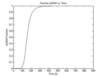
Fluorescence intensity is assumed to be proportional to the concentration of dsDNA. The magnitude of fluorescence intensity is the highest when all of the DNA is annealed, which corresponds to a value of 1 on the dsDNA fraction curve.
dsDnaFraction = DnaFraction(1E-6, T, -184, -71E3); % arguments: concentration,
                                                   % temp. vector, delta S, delta H
plot(t,dsDnaFraction)
title('Fraction dsDNA vs. Time');
xlabel('Time (s)');
ylabel('dsDNA Fraction');
Scale the curve and add some noise
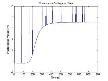
The output range of the transimpedance amplifier over the course of an experimental run can vary depending on several factors, including the amplifier gain, optical system gain, etc... A typical setup might produce values between, say, 0.5 and 7.2 Volts. The simulation code generates two random numbers to set the range and minimum value of the data. Your data analysis script will have to normalize the amplifier output voltage to a fractional value between 0 and 1. (What assumptions will you make about dsDNA concentration to do the normalization?)
In addition to Gaussian noise, the high gain amplifier can produce impulse noise. This can be caused by small static discharges, for example when a charged person sits down in a chair in the lab. It is a good idea to include some filtering for impulse noise in your data analysis script, in case your apparatus is susceptible to impulse noise.
Range = 5 + 4 * rand();                     % Range between 5 and 9
Minimum = 2 * rand() - 1;                   % Minimum between +/- 1
V_f = Range * f + Minimum;                  % Scale output
noise = 0.01 * randn(1,length(V_f));        % Random noise, standard deviation=10mV
V_f = V_f + noise;                          % Add random noise
noise = rand(1,length(V_f));                % Uniformly distributed  random numbers
ImpulseNoiseProbability = 1 ./ 75;          % Probability of impulse noise
noise = 20 * (noise < ImpulseNoiseProbability) - 10; % Quantize impulse noise
V_f = max(V_f, noise);                      % Add in impulse noise
plot(t, V_f)
title('Fluorescence Voltage vs. Time');
xlabel('Time (s)');
ylabel('Fluorescence Voltage (V)');
Reformat the data
When you import data from the LabView program that records DNA melting data, the format will be an N x 2 matrix with $ V_T $ values in column 1 and $ V_f $ in column 2. To put the simulated data in the same format, you can use Matlab's transpose operator (.') and the horizontal concatenation function horzcat:
simData = horzcat( V_RTD .', V_f .');
size(simData)


ans =

   901     2
Please see this page if you are uncertain about the .' operator.
Congratulations. You now have a simulated dataset that should be quite similar to what you measure in the lab.
Improving the model: photobleaching (optional)
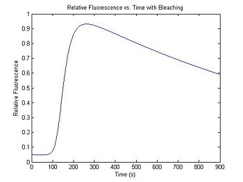
Each time a SYBR Green molecule absorbs a photon, there is a small chance that it will be destroyed and permanently lose its ability to fluoresce. The effect of photobleaching on the measured fluorescence intensity can be significant. To demonstrate this, a model for photobleaching may be added to the simulation. In the model, a small, fixed percentage of the fluorophores are mathematically destroyed each time sample. This simple difference equation can be implemented with a for...end loop.
- $ {f^\prime}_N = B f_{N-1} + f_N - f_{N-1} $
where,
- $ {f^\prime}_N $ is the Nth sample of the bleached relative fluorescence,
- $ \left . B \right . $ is a bleaching constant equal to the fraction of fluorophore not destroyed per time sample, and
- $ \left . f_N \right . $ is the Nth sample of the dsDNA fraction (relative fluorescence) curve.
The fraction of fluorophores destroyed per time sample is set by the variable bleachingConstant. In the example code, the constant is set so that half of the fluorophores will be destroyed over the course of the simulated experimental run.
bleachingConstant = (0.5)^(1/900);
diffDsDnaFraction = diff(dsDnaFraction);
dsDnaFractionBleached(1) = 0.05;
for ii = 2:length(dsDnaFraction)
    dsDnaFractionBleached(ii) = dsDnaFractionBleached(ii - 1) * ...
          bleachingConstant + diffDsDnaFraction(ii - 1);
end
plot(t,dsDnaFractionBleached)
title('Relative Fluorescence vs. Time with Bleaching');
xlabel('Time (s)');
ylabel('Relative Fluorescence');
The value of the first element of the vector dsDnaFractionBleached sets the initial condition for the differential equation — the relative fluorescence at the beginning of the simulation. Because SYBR green exhibits a small amount of intrinsic fluorescence when it is not bound to dsDNA, the initial value of dsDnaFractionBleached is set to a small number to model this effect.
Experiment with the bleaching constant and intrinsic fluorescence values to see how they distort the melting curve. Increasing the bleaching constant is equivalent to turning down the illumination intensity: fewer fluorphores will be destroyed in a given time. Unfortunately, the overall fluorescence intensity also decreases, necessitating higher amplifier gain and decreased signal to noise ratio. How will you decide on the optimal illumination and amplification levels in the lab? Can you use this model to correct for photobleaching effects in your data? How can you determine the bleaching constant experimentally?
If you would like to model photobleaching in your data analysis, follow the steps above for scaling the relative fluorescence signal, adding noise, and reformatting.
Data analysis advice
In outline, the steps to produce a melting curve from $ V_{RTD} $ and $ V_f $ are:
- Filter V_RTD and V_f to remove noise.
- Transform RTD voltage to temperature.
- Transform photodiode current to relative fluorescence.
- Ensure that the melting function is uniquely values by combining samples with identical temperature values.
- Differentiate the resulting function with respect to temperature.
Tm can be estimated directly from the melting curve or by finding the peak of the melting curve's derivative with respect to temperature. (Why would you prefer one method over the other?) Your data analysis script will have to convert the RTD and fluorescence intensity voltage signals into estimates of the temperature and dsDNA fraction.
Filtering
If you are not familiar with implementing digital filters in Matlab, review the Convolution and digital filtering in Matlab tutorial.
There are (at least)4 different convolution functions and 3 filtering functions in Matlab. Choosing the correct one is not always straightforward. Initial conditions Group delay
Uniquification
Sorting Binning
Numerical differentiation
diff function noise
