|
|
| Line 7: |
Line 7: |
| | | | |
| | ==Develop particle tracking code== | | ==Develop particle tracking code== |
| | + | Use the function <tt>SimulatedBrownianMotionMovie</tt> below to generate a synthetic movie of diffusing microspheres. You can use the synthetic movie and functions you developed in parts 1 and 2 to help you write code that will find centroids of the particles in each frame. Make sure to use the <tt>WeightedCentroid</tt> property instead of <tt>Centroid</tt> (and be sure you understand the difference between the two). Your function should return an N x 3 matrix of values where the first column is the Y coordinate, the second column is the X coordinate, and the third column is the frame number. |
| | | | |
| | + | <pre> |
| | + | function SimulatedMovie = SimulatedBrownianMotionMovie( varargin ) |
| | + | % this is a fancy way to take care of input arguments |
| | + | % all of the arguments have default values |
| | + | % if you want to change a default value, call this function with name/value pairs like this: |
| | + | % foo = SimulatedBrownianMotionMovie( 'NumerOfParticles', 10, 'ParticleDiameter' 3.2E-6 ); |
| | + | |
| | + | p = inputParser(); |
| | + | p.addParameter( 'NumberOfParticles', 5 ); |
| | + | p.addParameter( 'ParticleDiameter', 0.84E-6 ); |
| | + | p.addParameter( 'PixelSize', 7.4E-6 / 40 ); |
| | + | p.addParameter( 'ImageSize', [ 300 300 ] ); |
| | + | p.addParameter( 'FrameInterval', 1/10 ); |
| | + | p.addParameter( 'TemperatureKelvin', 293 ); |
| | + | p.addParameter( 'Viscosity', 1.0E-3 ); |
| | + | p.addParameter( 'BoltzmannConstant', 1.38e-23 ); |
| | + | p.addParameter( 'NumberOfFrames', 100 ); |
| | + | p.addParameter( 'ShowImages', true ); |
| | + | p.parse( varargin{:} ); |
| | + | |
| | + | assignLocalVariable = @( name, value ) assignin( 'caller', name, value ); |
| | + | allParameters = fields( p.Results ); |
| | + | |
| | + | for ii = 1:numel(allParameters) |
| | + | assignLocalVariable( allParameters{ii}, p.Results.(allParameters{ii}) ); |
| | + | end |
| | + | % at this point, there will be local scope variables with the names of |
| | + | % each of the parameters specified above |
| | + | |
| | + | close all |
| | + | |
| | + | diffusionCoefficient = BoltzmannConstant * TemperatureKelvin / ( 3 * pi * Viscosity * ParticleDiameter ); |
| | + | displacementStandardDeviation = sqrt( diffusionCoefficient * 2 * FrameInterval ); |
| | + | |
| | + | % create initial particle matrix |
| | + | particleRadiusInPixels = ParticleDiameter / 2 / PixelSize; |
| | + | particles = nan( NumberOfParticles, 4 ); |
| | + | particles(:, 1:2) = bsxfun( @times, rand( NumberOfParticles, 2 ), ImageSize ); |
| | + | particles(:, 3) = particleRadiusInPixels; |
| | + | particles(:, 4) = 4 * sqrt(2) * particleRadiusInPixels^2 * 4095; |
| | + | |
| | + | SimulatedMovie = zeros( ImageSize(1), ImageSize(2), NumberOfFrames ); |
| | + | figure |
| | + | |
| | + | for ii = 1:NumberOfFrames |
| | + | SimulatedMovie(:,:,ii) = SyntheticFluorescentMicrosphereImageWithNoise( particles, ImageSize ) / 4095; |
| | + | if( ShowImages ) |
| | + | imshow( SimulatedMovie(:,:,ii) ); |
| | + | drawnow |
| | + | end |
| | + | |
| | + | % update the particle position according to the diffusion |
| | + | % coefficient |
| | + | particles(:, 1:2) = particles(:, 1:2) + displacementStandardDeviation / PixelSize * randn( size( particles(:, 1:2) ) ); |
| | + | end |
| | + | end |
| | + | </pre> |
| | | | |
| − | | + | Once you have your N x 3 matrix, use the <tt>track</tt> function to add a fourth column to the matrix containing a unique identifier for each particle. The N x 4 matrix is an input to [[Calculating MSD and Diffusion Coefficients|this function for calculating MSD values and diffusion coefficients]]. |
| | | | |
| | ==Stability of microscope for particle tracking== | | ==Stability of microscope for particle tracking== |
| | + | Once you have developed and tested your code, use the following procedure to measure the location precision of your microscope: |
| | | | |
| − | The accuracy of optical particle tracking may be limited by mechanical and optical phenomena. Vibration and drift are a source of additive noise. [[Shot noise and centroid finding|Shot noise]] and CCD readout noise in the image of a particle bring about uncertainty in the estimate of its centroid. Excessive vibration can frequently be corrected by improving the mechanical support structure of the instrument. Most stages can be locked to reduce drift. Shot noise is fundamental; however, its relative contribution to the total signal can be minimized by ensuring that the optical system is functioning at peak efficiency.
| + | # Bring a slide with fixed beads into focus. |
| | + | **Choose a field of view in which you can see at least 3 beads using the 40× objective. |
| | + | ** Limit the field of view to only those beads by choosing a region of interest (ROI) in <tt>UsefulImageAcquisition</tt> tool. (Otherwise, you will have a gigantic movie that is hard to work with.) |
| | + | # Acquire a movie beads for 3 minutes at a frame rate of at least 10 fps. |
| | + | # Use the code you developed to track the particles and plot MSD versus time interval. |
| | | | |
| − | Before attempting to make measurements with particle tracking, it is essential to determine the performance characteristics of the instrument to be used. This can be accomplished by measuring a specimen with known characteristics. Perhaps the most foolproof choice is a sample with fixed particles. Any measured variation in the fixed sample is noise.
| + | [[Image:StabilityPlot2.jpg|right|400px|thumb|Your stability plot should look something like this.]] |
| − | | + | |
| − | In order to analyze your data, you will need to write code in Matlab. It is helpful to make sure your code is working before you collect data. '''Problem Set 2 will help you with this.''' You may download this set of Matlab files to help you get started: [[File:Matlab_Code_Following_Things_2.zip]]. Please note that you should take any code you download from the internet (including ones from this class) with a grain of salt--you will want to verify your code is working the way it should and that any bugs are fixed. One way to help test your code is to use it on simulated data, where you know what the output should be.
| + | |
| − | | + | |
| − | * To verify that your system is sufficiently stable for accurate particle tracking, monitor a dry specimen containing 0.84μm fluorescent beads.
| + | |
| − | | + | |
| − | [[Image:StabilityPlot2.jpg|right|400px|thumb|Example stability plot from Spring 2016 students.]] | + | |
| − | | + | |
| − | # Bring a slide with fixed beads into focus. Choose a field of view in which you can see at least 3 beads with the 40× objective. Limit the field of view to only those beads by choosing a region of interest (ROI) in <tt>UsefulImageAcquisition</tt> tool.
| + | |
| − | # Track the beads for 3 minutes (at least 20 fps) in a Matlab video and save the centroids with a frame rate of your choice and make a note of it.
| + | |
| − | # Use the Matlab function <code>track</code> (be sure to limit the algorithm to a small region of interest around the beads, otherwise Matlab will struggle!) to separate the centroids into individual trajectories, <math>\vec r_n(t)</math>, where <math>t = nT</math> and <math>T</math> is the inverse of the frame rate you set above.
| + | |
| − | <br>
| + | |
| − | | + | |
| − | * Use your data to calculate mean squared displacements [[MSD of Sum and Difference Trajectories|(MSDs) of sum and difference trajectories]]. You may have already completed this for Problem Set 2.
| + | |
| − | | + | |
| − | * Make any necessary adjustments to your microscope and repeat this particle-tracking procedure to attain sufficient stability:
| + | |
| − | The MSD from the difference trajectory should start out less than 100 nm<sup>2</sup> at t = 1 s and still be less than 1000 nm<sup>2</sup> for t = 180 s.
| + | |
| − | | + | |
| − | ===Particle Tracking===
| + | |
| − | | + | |
| − | In this part of the lab, you will follow microscopic objects throughout a series of movie frames: small, fluorescent microspheres first diffusing in purely viscous solutions of glycerol-water, and next moving in fibroblast cells after endocytosis.
| + | |
| − | Calculating the mean squared displacement of their motion as a function of time interval will allow you to characterize their physical environment and behavior, first in terms of diffusivity and viscosity coefficients of the glycerol-water mixtures, next recognizing other material or transport properties in fibroblast cells.
| + | |
| − | | + | |
| − | ====Contextual background====
| + | |
| − | ======Brownian motion======
| + | |
| − | This section was adapted from http://labs.physics.berkeley.edu/mediawiki/index.php/Brownian_Motion_in_Cells.
| + | |
| − | | + | |
| − | If you have ever looked at an aqueous sample through a microscope, you have probably noticed that every small particle you see wiggles about continuously. Robert Brown, a British botanist, was not the first person to observe these motions, but perhaps the first person to recognize the significance of this observation. Experiments quickly established the basic features of these movements. Among other things, the magnitude of the fluctuations depended on the size of the particle, and there was no difference between "live" objects, such as plant pollen, and things such as rock dust. Apparently, finely crushed pieces of an Egyptian mummy also displayed these fluctuations.
| + | |
| − | | + | |
| − | Brown noted: ''[The movements] arose neither from currents in the fluid, nor from its gradual evaporation, but belonged to the particle itself''.
| + | |
| − | | + | |
| − | This effect may have remained a curiosity had it not been for A. Einstein and M. Smoluchowski. They realized that these particle movements made perfect sense in the context of the then developing kinetic theory of fluids. If matter is composed of atoms that collide frequently with other atoms, they reasoned, then even relatively large objects such as pollen grains would exhibit random movements. This last sentence contains the ingredients for several Nobel prizes!
| + | |
| − | | + | |
| − | Indeed, Einstein's interpretation of Brownian motion as the outcome of continuous bombardment by atoms immediately suggested a direct test of the atomic theory of matter. Perrin received the 1926 Nobel Prize for validating Einstein's predictions, thus confirming the atomic theory of matter.
| + | |
| − | | + | |
| − | Since then, the field has exploded, and a thorough understanding of Brownian motion is essential for everything from polymer physics to biophysics, aerodynamics, and statistical mechanics. One of the aims of this lab is to directly reproduce the experiments of J. Perrin that lead to his Nobel Prize. A translation of the key work is included in the reprints folder. Have a look – he used latex spheres, and we will use polystyrene spheres, but otherwise the experiments will be identical. In addition to reproducing Perrin's results, you will probe further by looking at the effect of varying solvent molecule size.
| + | |
| − | | + | |
| − | ======Diffusion coefficient of microspheres in suspension======
| + | |
| − | According to theory,<ref>A. Einstein, [http://www.math.princeton.edu/~mcmillen/molbio/papers/Einstein_diffusion1905.pdf On the Motion of Small Particles Suspended in Liquids at Rest Required by the Molecular-Kinetic Theory of Heat], Annalen der Physik (1905).</ref><ref>E. Frey and K. Kroy, [http://www3.interscience.wiley.com/cgi-bin/abstract/109884431/ Brownian motion: a paradigm of soft matter and biological physics], Ann. Phys. (2005). Published on the 100th anniversary of Einstein’s paper, this reference chronicles the history of Brownian motion from 1905 to the present.</ref><ref>R. Newburgh, [http://scitation.aip.org/journals/doc/AJPIAS-ft/vol_74/iss_6/478_1.html Einstein, Perrin, and the reality of atoms: 1905 revisited], Am. J. Phys. (2006). A modern replication of Perrin's experiment. Has a good, concise appendix with both the Einstein and Langevin derivations.</ref><ref>M. Haw, [http://stacks.iop.org/JPhysCM/14/7769 Colloidal suspensions, Brownian motion, molecular reality: a short history], J. Phys. Condens. Matter (2002).</ref> the mean squared displacement of a suspended particle is proportional to the time interval as: <math>\left \langle {\left | \vec r(t+\tau)-\vec r(t) \right \vert}^2 \right \rangle=2Dd\tau</math>, where <i>r</i>(<i>t</i>) = position, <i>d</i> = number of dimensions, <i>D</i> = diffusion coefficient, and <math>\tau</math>= time interval.
| + | |
| − | | + | |
| − | ===Estimating the diffusion coefficient by tracking suspended microspheres===
| + | |
| − | | + | |
| − | [[Image: 20.309_130924_GlycerolChamber.png|right|thumb|200px|Imaging chamber for fluorescent microspheres diffusing in water:glycerol mixtures]]
| + | |
| − | 1. Track some 0.84μm Nile Red Spherotech polystyrene beads in water-glycerin mixtures (Samples A, B and C contain 0%, 30% and 50% glycerin, respectively).
| + | |
| − | | + | |
| − | :''Notes'': Fluorescent microspheres have been mixed for you by the instructors into water-glycerin solutions A, B, C, and D. (a) Vortex the stock Falcon tube, and then (b) transfer the bead suspension into its imaging chamber (consisting of a microscope slide, double-sided tape delimiting a 2-mm channel, and a 22x40mm No. 1.5 coverslip, and sealed at both ends nail polish).
| + | |
| − | | + | |
| − | :''Tip 1'': Do not choose to monitor particles that remain stably in focus: these are likely to be 'sitting on the coverslip' and their motion will not be representative of diffusion in the viscous water-glycerol fluid.
| + | |
| − | | + | |
| − | :''Tip 2'': Limit the ROI to a region with only 3 or 4 particles. Long movies with the whole field of view is a sure way to make MATLAB complain.
| + | |
| − | | + | |
| − | 2. Estimate the diffusion coefficient of these samples: MSD = <math>\left \langle {\left | \vec r(t+\tau)-\vec r(t) \right \vert}^2 \right \rangle=2Dd\tau</math>, where <i>r</i>(<i>t</i>) = position, <i>d</i> = number of dimensions, <i>D</i> = diffusion coefficient, and <math>\tau</math>= time interval. Use Sample A to verify that your algorithm correctly calculates the viscosity of water at the lab temperature (check the temperature on the clock on the wall or by other means).
| + | |
| − | :* '''Consider how many particles you should track and for how long. What is the uncertainty in your estimate?'''
| + | |
| − | :* '''From the viscosity calculation, estimate the glycerin/water weight ratio.''' (This [https://dl.dropboxusercontent.com/u/12957607/Viscosity%20of%20Aqueous%20Glycerine%20Solutions.pdf chart] is a useful reference. If that link doesn't work try [http://profs.engineering.uottawa.ca/biofluid/files/2011/08/viscosity-of-aqueous-glycerine-solutions.pdf this one].)
| + | |
| − | :* See: [http://labs.physics.berkeley.edu/mediawiki/index.php/Simulating_Brownian_Motion this page] for more discussion of Brownian motion and a Matlab simulation.
| + | |
| − | | + | |
| − | ===Live cell particle tracking of endocytosed beads===
| + | |
| − | | + | |
| − | We can also use particle tracking to probe cell samples. 0.84 μm diameter red fluorescent microspheres were mixed with the growth medium and added to the plated cells for a period of 12 to 24 hours for bead endocytosis.
| + | |
| − | | + | |
| − | You will be given two plates of cells for these experiments. The cells must be imaged while they are alive, so the cells must be used the day you are given them:
| + | |
| − | * <u>Dish 1</u> will be used to monitor particles in untreated cells, while
| + | |
| − | * <u>Dish 2</u> will be reserved to track microspheres after adding CytoD.
| + | |
| − | | + | |
| − | # Pre-warm your DMEM++ and CytoD to 37°C
| + | |
| − | # Carefully pipet out the medium from Dish 1. Gently rinse with 1mL of medium 2X to remove beads that were not endocytosed. Then, place 2 mL of fresh medium in dish.
| + | |
| − | # Choose cells in Dish 1 with at least 2 but preferably 3 or 4 particles embedded in them and capture movies of the samples. Make sure to do this quickly, as the cells become unhealthy without the temperature and carbon dioxide regulation.
| + | |
| − | #* By adjusting the LED current and exposure time, you should be able to use both bright field and fluorescence illumination simultaneously to find cells containing enough beads. Once you find a good-looking cell, turn off the LED and readjust the exposure time appropriately.
| + | |
| − | #* Take as many movies as you can with about 2-5 particles in the field of view in each movie.
| + | |
| − | # Next, carefully pipet out the medium in Dish 2. Gently rinse with 1mL of medium 2X to remove beads that were not endocytosed.
| + | |
| − | # Treat the cells in Dish 2 with the cytoskeleton-modifying CytoD: Pipet out remaining medium, add 1 mL pre-warmed CytoD solution at 10 μM (pre-mixed for you) to the dish, and incubate for 20 minutes at 37°C. It's a good idea to check on your cells after 15 minutes: sometimes they are in bad shape at that point but sometimes they still look very healthy. Wash 2X with 2 mL of pre-warmed DMEM++, leaving 2 mL in the dish when imaging.
| + | |
| − | # Perform and repeat the particle tracking measurements again in Dish 2 as quickly as you are able. It would be good to image the beads in only one cell at a time, since different cells may have different degrees of cytoskeletal disruption. Take as many videos as you can before the cells become sad. The cells' physiology has now been significantly disrupted by the toxin CytoD, and they will die within a couple of hours.
| + | |
| − | | + | |
| − | ==Report==
| + | |
| − | | + | |
| − | Find and follow all guidelines on the [[Microscopy report outline]] wiki page.
| + | |
| − | | + | |
| − | {{:Part 3 Combined Report Outline}}
| + | |
| − | | + | |
| − | {{:Optical microscopy lab wiki pages}}
| + | |
| | | | |
| | + | The MSD for the difference trajectory of two fixed particles should should start out less than 100 nm<sup>2</sup> and still be less than 1000 nm<sup>2</sup> for t = 180 s. If the MSD is larger than that, refine your apparatus and methodology until you achieve that goal. |
| | ==References== | | ==References== |
| − | * [http://www.youtube.com/watch?v=FAdxd2Iv-UA Random Force & Brownian Motion — 60 Symbols]
| |
| − |
| |
| | <References/> | | <References/> |
| | | | |
| | {{Template:20.309 bottom}} | | {{Template:20.309 bottom}} |
Overview
In this part of the assignment, you will develop code to track the positions of 0.84 μm fluorescent microspheres in a sequence of frames and determine the precision of position measurements with your microscope by tracking fixed microspheres. Next week, you will use the same code to characterize the diffusive motion of particles in different rheological environments (including live cells).
Develop particle tracking code
Use the function SimulatedBrownianMotionMovie below to generate a synthetic movie of diffusing microspheres. You can use the synthetic movie and functions you developed in parts 1 and 2 to help you write code that will find centroids of the particles in each frame. Make sure to use the WeightedCentroid property instead of Centroid (and be sure you understand the difference between the two). Your function should return an N x 3 matrix of values where the first column is the Y coordinate, the second column is the X coordinate, and the third column is the frame number.
function SimulatedMovie = SimulatedBrownianMotionMovie( varargin )
    % this is a fancy way to take care of input arguments
    % all of the arguments have default values
    % if you want to change a default value, call this function with name/value pairs like this:
    % foo = SimulatedBrownianMotionMovie( 'NumerOfParticles', 10, 'ParticleDiameter' 3.2E-6 );

    p = inputParser();
    p.addParameter( 'NumberOfParticles', 5 );
    p.addParameter( 'ParticleDiameter', 0.84E-6 );
    p.addParameter( 'PixelSize', 7.4E-6 / 40 );
    p.addParameter( 'ImageSize', [ 300 300 ] );
    p.addParameter( 'FrameInterval', 1/10 );
    p.addParameter( 'TemperatureKelvin', 293 );
    p.addParameter( 'Viscosity', 1.0E-3 );
    p.addParameter( 'BoltzmannConstant', 1.38e-23 );
    p.addParameter( 'NumberOfFrames', 100 );
    p.addParameter( 'ShowImages', true );
    p.parse( varargin{:} );

    assignLocalVariable = @( name, value ) assignin( 'caller', name, value );
    allParameters = fields( p.Results );

    for ii = 1:numel(allParameters)
        assignLocalVariable( allParameters{ii}, p.Results.(allParameters{ii}) );
    end
    % at this point, there will be local scope variables with the names of
    % each of the parameters specified above

    close all

    diffusionCoefficient = BoltzmannConstant * TemperatureKelvin / ( 3 * pi * Viscosity * ParticleDiameter );
    displacementStandardDeviation = sqrt( diffusionCoefficient * 2 * FrameInterval );

    % create initial particle matrix
    particleRadiusInPixels = ParticleDiameter / 2 / PixelSize;
    particles = nan( NumberOfParticles, 4 );
    particles(:, 1:2) = bsxfun( @times, rand( NumberOfParticles, 2 ), ImageSize );
    particles(:, 3) = particleRadiusInPixels;
    particles(:, 4) = 4 * sqrt(2) * particleRadiusInPixels^2 * 4095;

    SimulatedMovie = zeros( ImageSize(1), ImageSize(2), NumberOfFrames );
    figure

    for ii = 1:NumberOfFrames
        SimulatedMovie(:,:,ii) = SyntheticFluorescentMicrosphereImageWithNoise( particles, ImageSize ) / 4095;
        if( ShowImages )
            imshow( SimulatedMovie(:,:,ii) );
            drawnow
        end

        % update the particle position according to the diffusion
        % coefficient
        particles(:, 1:2) = particles(:, 1:2) + displacementStandardDeviation / PixelSize * randn( size( particles(:, 1:2) ) );
    end
end
Once you have your N x 3 matrix, use the track function to add a fourth column to the matrix containing a unique identifier for each particle. The N x 4 matrix is an input to this function for calculating MSD values and diffusion coefficients.
Stability of microscope for particle tracking
Once you have developed and tested your code, use the following procedure to measure the location precision of your microscope:
- Bring a slide with fixed beads into focus.
- Choose a field of view in which you can see at least 3 beads using the 40× objective.
- Limit the field of view to only those beads by choosing a region of interest (ROI) in UsefulImageAcquisition tool. (Otherwise, you will have a gigantic movie that is hard to work with.)
- Acquire a movie beads for 3 minutes at a frame rate of at least 10 fps.
- Use the code you developed to track the particles and plot MSD versus time interval.
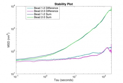
Your stability plot should look something like this.
The MSD for the difference trajectory of two fixed particles should should start out less than 100 nm2 and still be less than 1000 nm2 for t = 180 s. If the MSD is larger than that, refine your apparatus and methodology until you achieve that goal.
References

