Difference between revisions of "Assignment 2 Part 1: Noise in images"
(→Read noise and dark current noise) |
|||
| Line 141: | Line 141: | ||
As you can see from the plot, just due to chance alone, the number of photons emitted varies around the average value. Even though the average number of photons emitted and detected is constant, the actual number of photons is most often larger or smaller than the average. Due to the stochastic nature of photon emission, it is impossible to measure the average value without error in a finite amount of time. This kind of noise is called ''shot noise'' and it is inherent to the imaging process. | As you can see from the plot, just due to chance alone, the number of photons emitted varies around the average value. Even though the average number of photons emitted and detected is constant, the actual number of photons is most often larger or smaller than the average. Due to the stochastic nature of photon emission, it is impossible to measure the average value without error in a finite amount of time. This kind of noise is called ''shot noise'' and it is inherent to the imaging process. | ||
| − | + | Shot noise places a fundamental limit on the precision of light measurements. Even if you do everything exactly right, the signal to noise ratio of is | |
| + | |||
| + | :<math>\textrm{SNR}=\frac{N}{\sigma_N}=\frac{N}{\sqrt{N}}=\sqrt{N}</math> | ||
| + | |||
| + | An ideal detector is said to be ''shot noise limited'' and achieves an SNR of <math>\sqrt{N}</math> | ||
| + | |||
| + | ====Gaussian approximation==== | ||
| + | MATLAB can produce a lovely histogram of the simulation results: | ||
<pre> | <pre> | ||
| Line 174: | Line 181: | ||
==Read noise and dark current noise== | ==Read noise and dark current noise== | ||
[[File:Analog TV noise.jpg|right|thumb|Johnson noise on an old, analog television set.]] | [[File:Analog TV noise.jpg|right|thumb|Johnson noise on an old, analog television set.]] | ||
| − | |||
| − | + | On top of shot noise, most devices for measuring light like CCD and CMOS cameras has some additional shortcomings. Two important noise sources in cameras are ''dark current noise'' and ''read noise''. Both of these noises result from the way that electrons jiggle around in things that have a temperature above absolute zero. | |
| − | + | [[Image: 20.309 130827 DetectionLight3Stages.png|right|thumb|200 px|Detection of light]] | |
| + | * Detection of light can be decomposed in three simplified steps: | ||
| + | # conversion of light to free electrical charge-carriers | ||
| + | # conversion of current to voltage | ||
| + | # measurement of voltage. | ||
| + | |||
| + | Electrons in the detector don't have equal energies. Most of the electrons are at ground stat at normal temperatures. But just by chance, a few electrons will have energies high enough to make it into the bucket even though they were not excited by a photon. These "dark" electrons roll into the collection bucket and they are counted by The Count just the same as electrons that were excited by photons. Even in total darkness the count is not zero. Because there are a huge number of electrons and the probability that an electron will roll into the bucket without being excited by a photon is very small, the Poisson distribution is a good model for ''dark current''. Camera manufacturers frequently specify the ''dark current'' in units of electrons per pixel per second. The problem is not so much that dark electrons roll into the bucket — it's that the process is stochastic. The square root of the average number of dark electrons gives a good approximation for the standard deviation of the ''dark current noise''. | ||
| − | + | Another problem caused by thermal motion of electrons is called ''Johnson noise''. The electrons inside the resistor jiggle around stochastically. At any given time, a few more electrons jiggle left than right, and this gives rise to a noise voltage on the resistor if if there is no voltage applied. (Conceptually) electrons are counted by measuring the voltage they induce as they traverse a resistor. Johnson noise causes uncertainty in the counting process. The most frequently used model for Johnson is a Gaussian distribution. | |
In this section, you will add code to simulate these noise sources and redo the plots you did in the last section. | In this section, you will add code to simulate these noise sources and redo the plots you did in the last section. | ||
Revision as of 17:05, 18 September 2017
Overview
The process of recording a digital image is essentially an exercise in measuring the intensity of light at numerous points on a grid. Like most physical measurements, imaging is subject to measurement error. The formula below is a mathematical model of the imaging process, including noise and the camera's gain constant:
- $ P_{x,y} =G \left( I_{x,y} + \epsilon_{x,y} \right) $,
where $ x $ and $ y $ are spatial coordinates, $ P_{x,y} $ is the matrix of pixel values returned by the camera , $ G $ is the gain of the camera, $ I_{x,y} $ is the actual light intensity in the plane of the detector, and $ \epsilon_{x,y} $ is a matrix of error terms that represent noise introduced in the imaging process.
The amount of information in any signal, such as an image or a neural recording or a stock price, depends on the Signal to Noise Ratio (SNR). In this part of the assignment, you will develop a software model for imaging noise sources and you will use your model to explore how different noise sources affect image SNR.
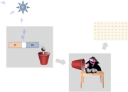
A (very) simplified model of digital image acquisition is shown in the image on the right. In the diagram, a luminous source stochastically emits $ \bar{N} $ photons per second. A fraction of the emitted photons lands on a semiconductor detector. Incident photons cause little balls (electrons) to fall out of the detector. The balls fall into a red bucket. At regular intervals, the bucket gets dumped out on to a table where the friendly muppet vampire Count von Count counts them. The process is repeated for each point on a grid. Not shown: the count is multiplied by a gain factor $ G $ before the array of measured values is returned to a recording device (such as a computer).
Before we dive into the computer model, it may be helpful to indulge in with a short review of (or introduction to) probability concepts.
Probability review
Random distributions
The question of what exactly a random variable is can get a bit philosophical. For present purposes, let's just say that a random variable represents the outcome of some stochastic process, and that you have no way to predict what the value of variable will be.
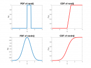
Even though the value of a random variable is not predictable, it is usually the case that some outcomes are more likely than others. The specification of the relative likelihood of each outcome is called a Probability Density Function (PDF), usually written as $ f_x(x) $. Two commonly-used PDFs are shown in the plots on the right. Larger values of the PDF indicate more likely outcomes.
The probability that a continuous random variable will take on a particular value such as 0.5 is (perhaps counter-intuitively) zero. This is because there are an infinite number of possible outcomes. The chance of getting exactly 0.5 when there are an infinite set of possible outcomes is equal to one divided by infinity. In other words, there is no chance at all of getting exactly 0.5. This is kind of baffling to think about and certainly annoying to work with. It's frequently cleaner to work with intervals. The chance that a random variable will fall between two numbers $ a $ and $ b $ can be found by integrating the PDF from $ a $ to $ b $:
- $ Pr(a \leq x \leq b)=\int_a^b f(x) $
The Cumulative Distribution Function $ F_x(x) $ is equal to the integral of the PDF from $ -\infty $ to $ x $:
- $ F_x(x)=\int_{-\infty}^x f_x(\tau) d\tau $
$ F_x(x) $ is the probability that $ x $ takes on a value less than $ x $. Using the CDF, it easy to calculate probability that $ x $ falls within the interval $ [a,b] $:
- $ Pr(a \leq x \leq b)=F_X(b)-F_x(a) $.
Mean, variance, and standard deviation
If you average a large number of outcomes of a random variable $ x $, the result approaches the variable's mean value $ \mu_x $:
- $ \lim_{N\to\infty} \frac{1}{N} \sum_{1}^{N}{x_n}=\mu_x $
The mean can also be found from the PDF by integrating every possible outcome multiplied by its likelihood:
- $ \mu_x=E(x)=\int_{−\infty}^{\infty}{x P(x) dx} $.
Standard deviation $ \sigma_x $ quantifies how far a random variable is likely to fall from its mean. Variance $ \sigma_x^2 $ is equal to the standard deviation squared. Sometimes, it is easier to work with variance in calculations. Most often, the interpretation of standard deviation is more intuitive than variance.
- $ \sigma_x^2=\lim_{N\to\infty} \frac{1}{N} \sum_{1}^{N}{(x_n-\mu_x)^2} $
Variance can also be calculated from the PDF:
- $ \sigma^2_x=\int_{−\infty}^{\infty}{(x-\mu)^2 P(x)dx} $
Calculations with random variables
If you add two random variables, their means add. Their variances also add. Standard deviations add under a big 'ol square root.
- $ \mu_{x+y}=\mu_x+\mu_y $
- $ \sigma_{x+y}^2=\sigma_x^2+\sigma_y^2 $
- $ \sigma_{x+y}=\sqrt{\sigma_x^2+\sigma_y^2} $
Averaging
If you average N independent outcomes of a random variable, the standard deviation of the average is equal to
- $ \sigma_{\bar{x},N}=\frac{\sigma_x}{\sqrt{N}} $
The standard deviation decreases in proportion to the square root of the number of averages. The term independent means that each outcome does not depend in any way on any other outcome.
Useful distributions
Binomial distribution
The binomial distribution considers the case where the outcome of a random variable is the sum of many individual go/no-go trials. The distribution assumes that the trials are independent and that the probability of success, $ p $, for each trial is the same. An example of a process that is well-modeled by the binomial distribution is the number of heads in 100 coin tosses. On each toss, the probability of success (heads) is $ p=0.5 $. If $ N $ is the number of trials, the average number of successes is equal to $ Np $. If you toss the coin 100 times, you expect on average to get 50 heads. The binomial distribution answers the question: "How surprised should I be if I get 12 heads?"[1] The probability mass function (PMF) for a random variable x ~ B(N, p) gives the probability of getting exactly k successes in N trials:
- $ Pr(k;n,p) = \Pr(x = k) = {n\choose k}p^k(1-p)^{n-k} $
for k = 0, 1, 2, ..., n, where
- $ \binom n k =\frac{n!}{k!(n-k)!} $
(This is called a PMF instead of a PDF because it is discrete — you can only get an integer between 0 and N if when counting the number of successes in N trials.)
The standard deviation of a binomial distribution is:
- $ \sigma_x^2=np(1-p) $
Poisson distribution
Sometimes, it is useful to model a binary process where you know the average value of the process, but not N and p. If p is small ($ p<<1 $), it is straightforward to make the approximation $ (1-p)=1 $. When p is small, a very good approximation of the variance is:
- $ \sigma_x^2=np $
The variance of a Poisson-distributed variable is equal to its mean. The Poisson distribution is a useful model for photon emission, radioactive decay, the number of letters you receive in the mail, the number of page requests on a certain website, the number of people who get in line to check out at a store, and many other everyday situations. The ability to estimate the variability of a binary process without knowing N and p is incredibly useful.
Normal distribution
The normal distribution (also frequently called a Gaussian distribution or a bell curve is specified by two parameters, an average value $ \mu $, and a standard deviation $ \sigma $:
- $ f(x \; | \; \mu, \sigma^2) = \frac{1}{\sqrt{2\pi\sigma^2} } \; e^{ -\frac{(x-\mu)^2}{2\sigma^2} } $
In the normal distribution, about 68% of outcomes fall within the interval $ \mu \pm \sigma $, about 95% in the interval $ \mu \pm 2 \sigma $, and about 99.7% in the interval $ \mu \pm 3 \sigma $
Central Limit Theorem
If you add together a bunch of independent random variables, their sum tends to look like a normal distribution
Modeling a single pixel
Let's start by modeling a single pixel. The first thing we need is a source of random numbers, so fire up MATLAB or any other computing you like on your computer (and stop whining about it). MATLAB includes several functions for generating random numbers. We will make our first model using the function rand(), which returns a random value that follows a uniform distribution in the interval (0, 1). Go ahead and type rand() at the command line. Matlab will return a number between 0 and 1. Do it a few times — it's kind of fun. You get a different number every single time. Can you guess what number will come next? If you can, please come see me.
If you want a bunch of random numbers, rand can help you out with that that, too. If you call rand with two integer M and N, the function will return a matrix of random numbers with M rows by N columns. The code snippet below to generates and displays (as an image) a 492 row x 656 column matrix of numbers with uniform distribution on the interval [0,1]:
noiseImage = rand( 492, 656 );
figure
imshow( noiseImage );
Okay, enough goofing around with the random number generator. Assume you are imaging a single molecule has a 0.01% chance of emitting a photon each microsecond. For the time being, assume you have perfect detector with a 100% chance of detecting each photon. The exposure (duration over which the measurement is made) is 1 second. To model photon emission over a single microsecond, you can use the rand function like this: sum( rand() < 0.000 )1. This statement will generate a vector of 1 million random numbers. The less than operator returns 1 for all values smaller than 10-4 and 0 for all the rest. Since rand returns numbers between 0 and 1 with a uniform distribution, there will be 0.01% chance of getting a 1 at any given position in the vector. The sum function adds up all of the ones and zeros and returns a count the total number of simulated photons emitted. On average, you would expect to detect about 100 photons during a one second long measurement. From what we know about the Poisson distribution, we can guess that the standard deviation will be very close to the square root of the average value, or about 10 in this case. The std function computes the standard deviation of its argument.
Let's run the simulation one thousand times and plot the results. You can copy-paste this code into the MATLAB command window.
close all
figure

probabilityOfEmission = 1E-4;
numberOfPhotonsEmitted = nan( 1, 1000 ); % allocate space for the results

for ii = 1:1000
    numberOfPhotonsEmitted(ii) = sum( ( rand( 1, 1E6 ) < probabilityOfEmission ) );
    plot( numberOfPhotonsEmitted, 'x' );
    axis( [ 1 1000 0 140 ] );
    xlabel( 'n' );
    ylabel( 'Number of Photons' );
    title( [ 'Photon Count (N=' num2str(ii) ...
        ' siumulations) \mu=' num2str( mean( numberOfPhotonsEmitted(1:ii) ) ) ...
        ' \sigma=' num2str( std( numberOfPhotonsEmitted(1:ii) ) )] );
    drawnow
end
As you can see from the plot, just due to chance alone, the number of photons emitted varies around the average value. Even though the average number of photons emitted and detected is constant, the actual number of photons is most often larger or smaller than the average. Due to the stochastic nature of photon emission, it is impossible to measure the average value without error in a finite amount of time. This kind of noise is called shot noise and it is inherent to the imaging process.
Shot noise places a fundamental limit on the precision of light measurements. Even if you do everything exactly right, the signal to noise ratio of is
- $ \textrm{SNR}=\frac{N}{\sigma_N}=\frac{N}{\sqrt{N}}=\sqrt{N} $
An ideal detector is said to be shot noise limited and achieves an SNR of $ \sqrt{N} $
Gaussian approximation
MATLAB can produce a lovely histogram of the simulation results:
edges = 40:10:160;
centers = ( edges(1:(end-1)) + edges(2:end) ) / 2;
[ counts ] = histcounts( numberOfPhotonsEmitted, edges );
figure
bar( centers, counts )

% add numbers on top of the bars
for ii=1:numel(centers)
    text( centers(ii), counts(ii), num2str( counts(ii) ),...
               'HorizontalAlignment','center',...
               'VerticalAlignment','bottom')
end

title( 'Distribution of Simulated Photon Counts' )
ylabel( 'Number of Results in Range' )
xlabel( 'Number of Photons' )
Read noise and dark current noise
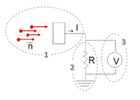
On top of shot noise, most devices for measuring light like CCD and CMOS cameras has some additional shortcomings. Two important noise sources in cameras are dark current noise and read noise. Both of these noises result from the way that electrons jiggle around in things that have a temperature above absolute zero.
- Detection of light can be decomposed in three simplified steps:
- conversion of light to free electrical charge-carriers
- conversion of current to voltage
- measurement of voltage.
Electrons in the detector don't have equal energies. Most of the electrons are at ground stat at normal temperatures. But just by chance, a few electrons will have energies high enough to make it into the bucket even though they were not excited by a photon. These "dark" electrons roll into the collection bucket and they are counted by The Count just the same as electrons that were excited by photons. Even in total darkness the count is not zero. Because there are a huge number of electrons and the probability that an electron will roll into the bucket without being excited by a photon is very small, the Poisson distribution is a good model for dark current. Camera manufacturers frequently specify the dark current in units of electrons per pixel per second. The problem is not so much that dark electrons roll into the bucket — it's that the process is stochastic. The square root of the average number of dark electrons gives a good approximation for the standard deviation of the dark current noise.
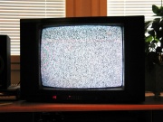
Another problem caused by thermal motion of electrons is called Johnson noise. The electrons inside the resistor jiggle around stochastically. At any given time, a few more electrons jiggle left than right, and this gives rise to a noise voltage on the resistor if if there is no voltage applied. (Conceptually) electrons are counted by measuring the voltage they induce as they traverse a resistor. Johnson noise causes uncertainty in the counting process. The most frequently used model for Johnson is a Gaussian distribution.
In this section, you will add code to simulate these noise sources and redo the plots you did in the last section.
This happens because the temperature of the detector is not at absolute zero. Just by chance there will be a few electrons with enough thermal energy to make it into the bucket. This is called dark current.
Another problem comes up when you try to count the electrons.
A few balls roll out of the detector and into the bucket and they are because a few electrons in the detector have high energy just by chance because the temperature of the detector is not zero.
Binomial and Poisson distributions
This kind of thing comes up quite a lot — where you have a bunch of identical events and each event either occurs or does not occur with a given probability $ p $. There is no possibility that the event half-occurs, so the event count will always take on an integer value. One of the best-known examples of this is a coin toss. Assuming the coin is fair, the probability of the event occurring (say, heads) $ p=0.5 $. If you flip a coin 100 times,
Referneces
- ↑ Answer: extremely surprised. The probability of this happening is about 10-15
- Overview
- Part 1: Noise in images
- Part 2: Fluorescence microscopy
- Part 3: Build an epi-illuminator for your microscope
Back to 20.309 Main Page


