Difference between revisions of "Assignment 2 Part 1: Noise in images"
(→Probability review) |
(→Probability review) |
||
| Line 19: | Line 19: | ||
==Probability review== | ==Probability review== | ||
| + | ===Random variable distributions=== | ||
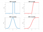
[[File:PDF and CDF of MATLAB rand and randn functions.png|thumb|right|Plots of PDF <math>f_x(x)</math> vs. <math>x</math> and CDF <math>F_x(x)</math> vs <math>x</math> for the uniform distribution on the interval (0,1) and the normal distribution with <math>\mu=0</math> and <math>\sigma=1</math>. MATLAB functions <tt>rand</tt> and <tt>randn</tt> return pseudorandom values that follow these distributions.]] | [[File:PDF and CDF of MATLAB rand and randn functions.png|thumb|right|Plots of PDF <math>f_x(x)</math> vs. <math>x</math> and CDF <math>F_x(x)</math> vs <math>x</math> for the uniform distribution on the interval (0,1) and the normal distribution with <math>\mu=0</math> and <math>\sigma=1</math>. MATLAB functions <tt>rand</tt> and <tt>randn</tt> return pseudorandom values that follow these distributions.]] | ||
The question of what exactly a random variable is can get a bit philosophical. For present purposes, let's just say that a random variable represents the outcome of some stochastic process, and that you have no way to predict what the value of variable will be. | The question of what exactly a random variable is can get a bit philosophical. For present purposes, let's just say that a random variable represents the outcome of some stochastic process, and that you have no way to predict what the value of variable will be. | ||
| Line 32: | Line 33: | ||
:<math>F_x(x)=\int_{-\infty}^x f_x(\tau) d\tau</math> | :<math>F_x(x)=\int_{-\infty}^x f_x(\tau) d\tau</math> | ||
| − | <math>F_x(x)</math> is the probability that <math>x</math> takes on a value less than <math>x</math>. The probability that <math>x</math> falls within the interval <math>[a,b]</math> | + | <math>F_x(x)</math> is the probability that <math>x</math> takes on a value less than <math>x</math>. The CDF makes it easy to calculate probability that <math>x</math> falls within the interval <math>[a,b]</math>: <math>:Pr(a \leq x \leq b)=F_X(b)-F_x(a)</math>. |
| + | ===Measures of central tendency and dispersion=== | ||
If you know the PDF, you can calculate the expected (or mean) value <math>\mu</math> and variance <math>\sigma^2</math> of a random variable. These are given by: | If you know the PDF, you can calculate the expected (or mean) value <math>\mu</math> and variance <math>\sigma^2</math> of a random variable. These are given by: | ||
| Line 39: | Line 41: | ||
:<math>\sigma^2=\int_{−\infty}^{\infty}{(x-\mu)^2 P(x)dx}</math> | :<math>\sigma^2=\int_{−\infty}^{\infty}{(x-\mu)^2 P(x)dx}</math> | ||
| − | Mean is a way to measure of the ''central tendency'' of a distribution and standard deviation is a measure of its ''spread''. If you evaluated the random variable a large number of times and averaged all the outcomes, the average would tend to approach <math>\mu</math>. Standard deviation (the square root of variance) gives a sense of how far an outcome is likely to lie from the mean. | + | Mean is a way to measure of the ''central tendency'' of a distribution and standard deviation is a measure of its ''dispersion'' or ''spread''. If you evaluated the random variable a large number of times and averaged all the outcomes, the average would tend to approach <math>\mu</math>. ''Standard deviation'' (the square root of variance) gives a sense of how far an outcome is likely to lie from the mean. |
| + | |||
| + | ===Calculations with random variables=== | ||
| + | If you add two random variables, their means add. Their variances also add. Standard deviations add under a big 'ol square root. | ||
| + | |||
| + | :<math>\mu_{x+y}=\mu_x+\mu_y</math> | ||
| + | :<math>\sigma_{x+y}^2=\sigma_x^2+\sigma_y^2</math> | ||
| + | :<math>\sigma_{x+y}=\sqrt{\sigma_x^2+\sigma_y^2}</math> | ||
==Modeling photon emission== | ==Modeling photon emission== | ||
Revision as of 14:45, 17 September 2017
Overview
The process of recording a digital image is essentially an exercise in measuring the intensity of light at numerous points on a grid. Like most physical measurements, imaging is subject to measurement error. The formula below is a mathematical model of the imaging process, including noise and the camera's gain constant:
- $ P_{x,y} =G \left( I_{x,y} + \epsilon_{x,y} \right) $,
where $ x $ and $ y $ are spatial coordinates, $ P_{x,y} $ is the matrix of pixel values returned by the camera , $ G $ is the gain of the camera, $ I_{x,y} $ is the actual light intensity in the plane of the detector, and $ \epsilon_{x,y} $ is a matrix of error terms that represent noise introduced in the imaging process.
The amount of information in any signal, such as an image or a neural recording or a stock price, depends on the Signal to Noise Ratio (SNR). In this part of the assignment, you will develop a software model for imaging noise sources and you will use your model to explore how different noise sources affect image SNR.
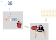
A (very) simplified model of digital image acquisition is shown in the image on the right. In the diagram, a luminous source stochastically emits $ \bar{N} $ photons per second. A fraction of the emitted photons lands on a semiconductor detector. Incident photons cause little balls (electrons) to fall out of the detector. The balls fall into a red bucket. At regular intervals, the bucket gets dumped out on to a table where the friendly muppet vampire Count von Count counts them. The process is repeated for each point on a grid. Not shown: the count is multiplied by a gain factor $ G $ before the array of measured values is returned to a recording device (such as a computer).
Before we dive into the computer model, it may be helpful to indulge in with a short review of (or introduction to) probability concepts.
Probability review
Random variable distributions
The question of what exactly a random variable is can get a bit philosophical. For present purposes, let's just say that a random variable represents the outcome of some stochastic process, and that you have no way to predict what the value of variable will be.
Even though the value of a random variable is not predictable, it is usually the case that some outcomes are more likely than others. The specification of the relative likelihood of each outcome is called a Probability Density Function (PDF), usually written as $ f_x(x) $. Two commonly-used PDFs are shown in the plots on the right. Larger values of the PDF indicate more likely outcomes.
Perhaps counterintuitively, the PDF doesn't really tell you how likely a certain outcome is. The probability that a continuous random variable will take on a particular value such as 0.5 is zero. This is because there are an infinite number of possible outcomes. The chance of getting 0.5 when there are an infinite set of possible outcomes is equal to one divided by infinity. In other words, there is no chance at all of getting exactly 0.5. This is kind of baffling to think about and certainly annoying to work with. It's usually cleaner to think about a random variable falling within a certain interval. The chance that a random variable will fall between two numbers $ a $ and $ b $ can be found by integrating the PDF from $ a $ to $ b $:
- $ Pr(a \leq x \leq b)=\int_a^b f(x) $
Since probability calculations so frequently use the integral of the PDF, whoever decides these things defined a function called the Cumulative Distribution Function $ F_X(x) $ that is equal to the integral of the PDF from $ -\infty $ to $ x $:
- $ F_x(x)=\int_{-\infty}^x f_x(\tau) d\tau $
$ F_x(x) $ is the probability that $ x $ takes on a value less than $ x $. The CDF makes it easy to calculate probability that $ x $ falls within the interval $ [a,b] $: $ :Pr(a \leq x \leq b)=F_X(b)-F_x(a) $.
Measures of central tendency and dispersion
If you know the PDF, you can calculate the expected (or mean) value $ \mu $ and variance $ \sigma^2 $ of a random variable. These are given by:
- $ \mu=E(X)=\int_{−\infty}^{\infty}{x P(x) dx} $
- $ \sigma^2=\int_{−\infty}^{\infty}{(x-\mu)^2 P(x)dx} $
Mean is a way to measure of the central tendency of a distribution and standard deviation is a measure of its dispersion or spread. If you evaluated the random variable a large number of times and averaged all the outcomes, the average would tend to approach $ \mu $. Standard deviation (the square root of variance) gives a sense of how far an outcome is likely to lie from the mean.
Calculations with random variables
If you add two random variables, their means add. Their variances also add. Standard deviations add under a big 'ol square root.
- $ \mu_{x+y}=\mu_x+\mu_y $
- $ \sigma_{x+y}^2=\sigma_x^2+\sigma_y^2 $
- $ \sigma_{x+y}=\sqrt{\sigma_x^2+\sigma_y^2} $
Modeling photon emission
In this part of the assignment, you will make a computer model of the process of measuring light in order to examine how noise sources affect images. Photon emission is a stochastic process, so we will start with a short review of (or introduction to) some probability concepts. It's time to fire up MATLAB. Feel free to use a another language, if you like. The commands are very similar in most languages.
We are going to model a stochastic process, so the first thing we need is a source of random numbers. MATLAB includes several functions for generating random numbers. We will to make our first model using the function rand(), which returns a random value that follows a uniform distribution in the interval (0, 1). Go ahead and type rand() at the command line. Matlab will return a number between 0 and 1. Do it a few times — it's kind of fun. Can you guess what number will come next? If you can, please come see me. If you want more than one random number, you can pass that information to rand with arguments. For example, try the code snippet below to generate and display (as an image) a matrix with 492 rows x 656 columns of numbers between 0 and 1:
totallyNoisyImage = rand( 492, 656 );
figure
imshow( totallyNoisyImage );
figure
hist( totallyNoiseImage(:) );
- Overview
- Part 1: Noise in images
- Part 2: Fluorescence microscopy
- Part 3: Build an epi-illuminator for your microscope
Back to 20.309 Main Page


